
最近我们被客户要求撰写关于面板平滑转换回归(PSTR)的研究报告。建模过程包括三个阶段:表述,估计和评估。
本文帮助用户进行模型表述、估计,进行PSTR模型评估。在程序包中实现了集群依赖性和异方差性一致性检验。
可下载资源
还实现了wild bootstrap和cluster wild bootstrap检验。
并行计算(作为选项)在某些函数中实现,尤其是bootstrap检验。因此,该程序包适合在超级计算服务器上运行多个核心的任务。
数据
本文使用“Hansen99”数据集来提供示例。

初始化
可以通过执行创建PSTR类的新对象
#> Summary of the model:
#> ---------------------------------------------------------------------------
#>   time horizon sample size = 14,  number of individuals = 560
#> ---------------------------------------------------------------------------
#> Dependent variable:  inva
#> ---------------------------------------------------------------------------
#> Explanatory variables in the linear part:
#>   dt_75 dt_76 dt_77 dt_78 dt_79 dt_80 dt_81 dt_82 dt_83 dt_84 dt_85 dt_86 dt_87 vala debta cfa sales
#> ---------------------------------------------------------------------------
#> Explanatory variables in the non-linear part:
#>   vala debta cfa sales
#> ---------------------------------------------------------------------------
#> Potential transition variable(s) to be tested:
#>   vala
#> ###########################################################################
#> ***************************************************************************
#> Results of the linearity (homogeneity) tests:
#> ***************************************************************************
#> Sequence of homogeneity tests for selecting number of switches 'm':
因变量是“inva”,第4列到第20列的数据中的变量是线性部分的解释变量,非线性部分中的解释变量是“indep_k”中的四个,潜在的转换变量是“vala”(Tobin的Q)。
以下代码执行线性检验
#> Results of the linearity (homogeneity) tests:
#> ---------------------------------------------------------------------------
#> LM tests based on transition variable 'vala'
#>   m  LM_X PV  LM_F PV HAC_X        PV HAC_F        PV
#>   1 125.3  0 28.99  0 30.03 4.819e-06 6.952 1.396e-05
#> ***************************************************************************
#> Sequence of homogeneity tests for selecting number of switches 'm':
#> ---------------------------------------------------------------------------
#> LM tests based on transition variable 'vala'
#>   m  LM_X PV  LM_F PV HAC_X        PV HAC_F        PV
#>   1 125.3  0 28.99  0 30.03 4.819e-06 6.952 1.396e-05
可以看到函数“LinTest”获取PSTR对象“pstr”并返回结果。因为处理包中PSTR对象的函数通过添加新的atrributes来更新对象。当然可以创建新的PSTR对象来获取返回值,以便保存模型的不同设置的结果。
可以通过运行以下代码来执行wild bootstrap和wild cluster bootstrap。
估计
当确定要用于估计的转换变量时,在本例中为“inva”,可以估计PSTR模型
print(pstr,"estimates")默认情况下,使用“optim”方法“L-BFGS-B”,但可以通过更改优化方法进行估算
 print(pstr,"estimates")
***************************************************************************
#> Results of the PSTR estimation:
#> ---------------------------------------------------------------------------
#> Transition variable 'vala' is used in the estimation.
#> ---------------------------------------------------------------------------
#> Parameter estimates in the linear part (first extreme regime) are
#>        dt_75_0   dt_76_0   dt_77_0   dt_78_0  dt_79_0  dt_80_0   dt_81_0
#> Est  -0.002827 -0.007512 -0.005812 0.0003951 0.002464 0.006085 0.0004164
#> s.e.  0.002431  0.002577  0.002649 0.0027950 0.002708 0.002910 0.0029220
#>        dt_82_0   dt_83_0    dt_84_0  dt_85_0   dt_86_0   dt_87_0  vala_0
#> Est  -0.007802 -0.014410 -0.0009146 0.003467 -0.001591 -0.008606 0.11500
#> s.e.  0.002609  0.002701  0.0030910 0.003232  0.003202  0.003133 0.04073
#>       debta_0   cfa_0  sales_0
#> Est  -0.03392 0.10980 0.002978
#> s.e.  0.03319 0.04458 0.008221
#> ---------------------------------------------------------------------------
#> Parameter estimates in the non-linear part are
#>        vala_1 debta_1    cfa_1  sales_1
#> Est  -0.10370 0.02892 -0.08801 0.005945
#> s.e.  0.03981 0.04891  0.05672 0.012140
#> ---------------------------------------------------------------------------
#> Parameter estimates in the second extreme regime are
#>      vala_{0+1} debta_{0+1} cfa_{0+1} sales_{0+1}
#> Est    0.011300    -0.00500   0.02183    0.008923
#> s.e.   0.001976     0.01739   0.01885    0.004957
#> ---------------------------------------------------------------------------
#> Non-linear parameter estimates are
#>       gamma        c_1
#> Est  0.6299 -0.0002008
#> s.e. 0.1032  0.7252000
#> ---------------------------------------------------------------------------
#> Estimated standard deviation of the residuals is 0.04301
#> 还实现了线性面板回归模型的估计。
 print(pstr0,"estimates")
#> ###########################################################################
#> ## PSTR 1.2.4 (Orange Panel)
#> ###########################################################################
#> ***************************************************************************
#> A linear panel regression with fixed effects is estimated.
#> ---------------------------------------------------------------------------
#> Parameter estimates are
#>          dt_75     dt_76     dt_77    dt_78    dt_79    dt_80    dt_81
#> Est  -0.007759 -0.008248 -0.004296 0.002356 0.004370 0.008246 0.004164
#> s.e.  0.002306  0.002544  0.002718 0.002820 0.002753 0.002959 0.002992
#>          dt_82     dt_83    dt_84    dt_85    dt_86     dt_87     vala
#> Est  -0.005294 -0.010040 0.006864 0.009740 0.007027 0.0004091 0.008334
#> s.e.  0.002664  0.002678 0.003092 0.003207 0.003069 0.0030080 0.001259
#>          debta     cfa    sales
#> Est  -0.016380 0.06506 0.007957
#> s.e.  0.005725 0.01079 0.002412
#> ---------------------------------------------------------------------------
#> Estimated standard deviation of the residuals is 0.04375
#> ***************************************************************************
#> ###########################################################################
评估
可以基于估计的模型进行评估测试

请注意,在“EvalTest”中,每次只有一个转换变量用于非线性测试。这与“LinTest”函数不同,后者可以采用多个转换变量。这就是为什么我将结果保存到新的PSTR对象“pstr1”而不是覆盖的原因。通过这样做,我可以在新对象中保存来自不同转换变量的更多测试结果。
iB = 5000
cpus = 50

## wild bootstrap time-varyint评估检验
pstr = WCB_TVTest(use=pstr,iB=iB,parallel=T,cpus=cpus)

## wild bootstrap异质性评估检验
pstr1 = WCB_HETest(use=pstr1,vq=pstr$mQ[,1],iB=iB,parallel=T,cpus=cpus)
请注意,评估函数不接受线性面板回归模型中返回的对象“pstr0”,因为评估测试是针对估计的PSTR模型设计的,而不是线性模型。
可视化
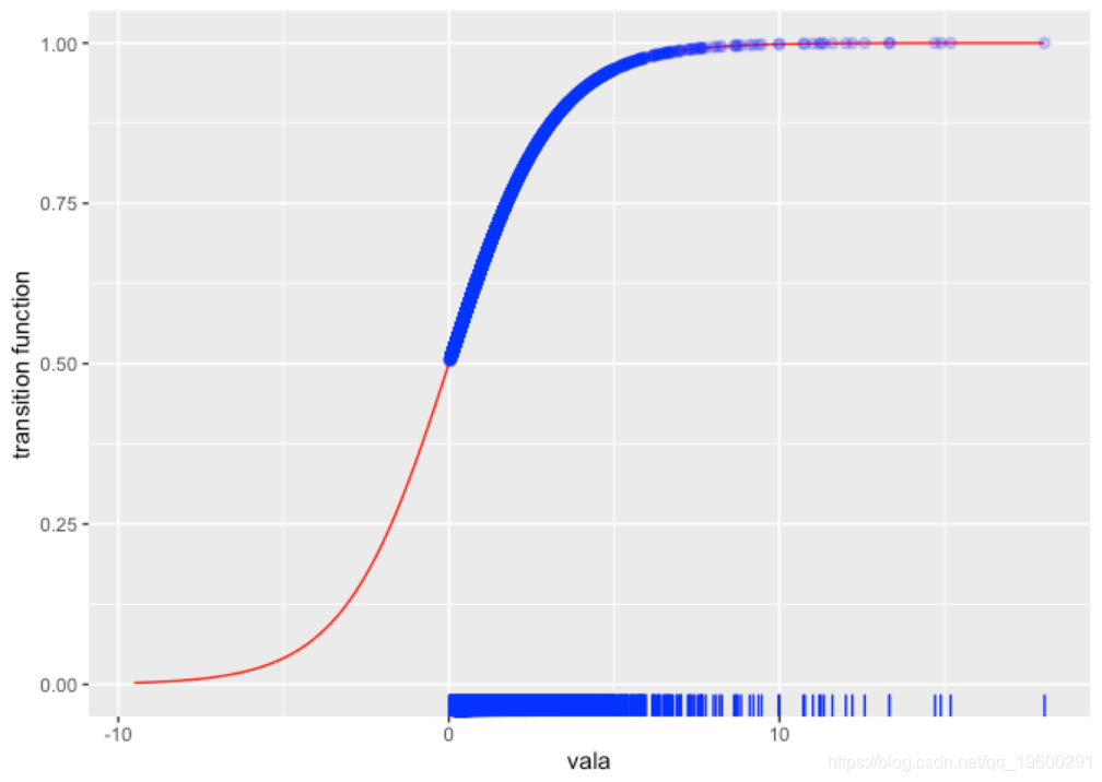
估算PSTR模型后,可以绘制估计的转换函数
随时关注您喜欢的主题
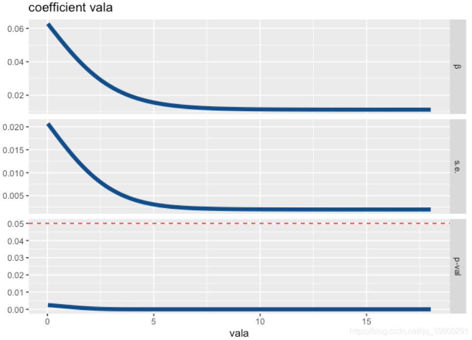
还可以根据转换变量绘制系数曲线,标准误差和p值。
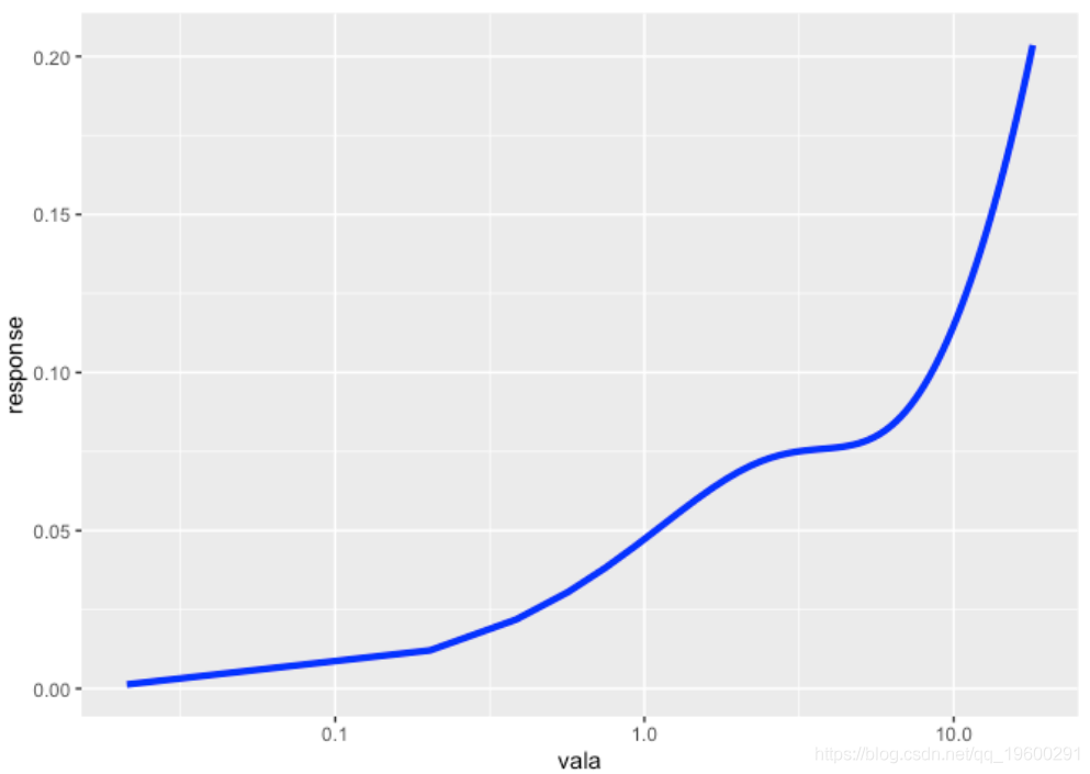
绘图函数plot_response,描述了PSTR模型的因变量和一些解释性变量。
我们可以看到,如果没有非线性,对变量的响应是一条直线。如果变量和转换变量是不同的,我们可以绘制曲面,z轴为响应,x轴和y轴为两个变量。如果变量和转换变量相同,则变为曲线。
我们通过运行来制作图表
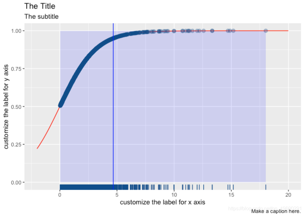
x轴上的数字看起来不太好,因为很难找到转折点的位置。
该ggplot2软件包允许我们手动绘制数字。
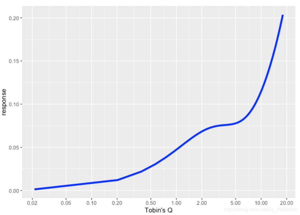
现在我们非常清楚地看到,大约0.5的转折点将曲线切割成两种状态,并且两种状态的行为完全不同。该图表是关于托宾Q对预期投资的滞后影响。低Q值公司(其潜力被金融市场评估为低)可能不太愿意改变他们未来的投资计划,或者可能会改变。
 R语言Stan贝叶斯回归置信区间后验分布可视化模型检验
 R语言分类回归分析考研热现象分析与考研意愿价值变现
 SPSS用多元逐步回归模型对上证指数预测、描述统计和相关分析可视化研究
 R语言、WEKA关联规则、决策树、聚类、回归分析工业企业创新情况影响因素数据


1 comment on “R语言面板平滑转换回归(PSTR)分析案例实现”