在逻辑回归中，我们将二元因变量Y_i回归到协变量X_i上。

由Kaizong Ye，Weilong Zhang撰写

下面的代码使用Metropolis采样来探索 beta_1和beta_2 的后验Yi到协变量Xi。

定义expit和分对数链接函数，此函数计算beta_1，beta_2的联合后验。

可下载资源

完整程序、数据和文档（word）

它返回后验的对数以获得数值稳定性。

一般来说M-H采样算法较MCMC算法应用更广泛，然而在大数据时代，M-H算法面临着两个问题：

1）在高维时的计算量很大，算法效率很低，同时存在拒绝转移的问题，也会加大计算量

2）由于特征维度大，很多时候我们甚至很难求出目标的各特征维度联合分布，但是可以方便求出各个特征之间的条件概率分布（因此就思考是否能只知道条件概率分布的情况下进行采样）。

logit<-function(x){log(x/(1-x))} 
log_post<-function(Y,X,beta){
    prob1  <- expit(beta[1] + beta[2]*X)
like+prior}

这是MCMC的主要功能.can.sd是候选标准偏差。

Bayes.logistic<-function(y,X,
                         n.samples=10000,
                         can.sd=0.1){

     keep.beta     <- matrix(0,n.samples,2)
     keep.beta[1,] <- beta

     acc   <- att <- rep(0,2)

    for(i in 2:n.samples){

      for(j in 1:2){

       att[j] <- att[j] + 1

      # 抽取候选:

       canbeta    <- beta
       canbeta[j] <- rnorm(1,beta[j],can.sd)
       canlp      <- log_post(Y,X,canbeta)

      # 计算接受率:

       R <- exp(canlp-curlp)  
       U <- runif(1)                          
       if(U<R){       
          acc[j] <- acc[j]+1
       }
     }
     keep.beta[i,]<-beta

   }
   # 返回beta的后验样本和Metropolis的接受率


list(beta=keep.beta,acc.rate=acc/att)}

视频

逻辑回归Logistic模型原理和R语言分类预测冠心病风险实例

探索见解 ➜

去bilibili观看 ➜

探索更多视频 ➜

生成模拟数据

 set.seed(2008)
 n         <- 100
 X         <- rnorm(n)
  true.p    <- expit(true.beta[1]+true.beta[2]*X)
 Y         <- rbinom(n,1,true.p)

拟合模型

 burn      <- 10000
 n.samples <- 50000
  fit  <- Bayes.logistic(Y,X,n.samples=n.samples,can.sd=0.5)
 tock <- proc.time()[3]

 tock-tick

##    3.72

结果

abline(true.beta[1],0,lwd=2,col=2)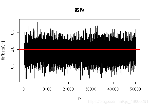

最受欢迎的见解

1.使用R语言进行METROPLIS-IN-GIBBS采样和MCMC运行

2.R语言中的Stan概率编程MCMC采样的贝叶斯模型

3.R语言实现MCMC中的Metropolis–Hastings算法与吉布斯采样

4.R语言BUGS JAGS贝叶斯分析马尔科夫链蒙特卡洛方法（MCMC）采样

5.R语言中的block Gibbs吉布斯采样贝叶斯多元线性回归

6.R语言Gibbs抽样的贝叶斯简单线性回归仿真分析

7.R语言用Rcpp加速Metropolis-Hastings抽样估计贝叶斯逻辑回归模型的参数

8.R语言使用Metropolis- Hasting抽样算法进行逻辑回归

9.R语言中基于混合数据抽样(MIDAS)回归的HAR-RV模型预测GDP增长

abline(true.beta[2],0,lwd=2,col=2)

R语言Gibbs抽样的贝叶斯简单线性回归仿真分析

阅读文章 ➜

 hist(fit$beta[,1],main="Intercept",xlab=expression(beta[1]),breaks=50)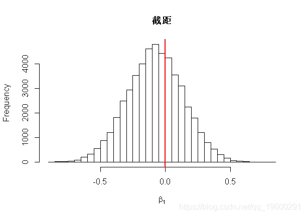

随时关注您喜欢的主题

 abline(v=true.beta[2],lwd=2,col=2)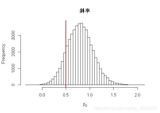

 print("Posterior mean/sd")
## [1] "Posterior mean/sd"
 print(round(apply(fit$beta[burn:n.samples,],2,mean),3))
## [1] -0.076  0.798
 print(round(apply(fit$beta[burn:n.samples,],2,sd),3))
## [1] 0.214 0.268

## 
## Deviance Residuals: 
##     Min       1Q   Median       3Q      Max  
## -1.6990  -1.1039  -0.6138   1.0955   1.8275  
## 
## Coefficients:
##             Estimate Std. Error z value Pr(>|z|)   
## (Intercept) -0.07393    0.21034  -0.352  0.72521   
## X            0.76807    0.26370   2.913  0.00358 **
## ---
## Signif. codes:  0 '***' 0.001 '**' 0.01 '*' 0.05 '.' 0.1 ' ' 1
## 
## (Dispersion parameter for binomial family taken to be 1)
## 
##     Null deviance: 138.47  on 99  degrees of freedom
## Residual deviance: 128.57  on 98  degrees of freedom
## AIC: 132.57
## 
## Number of Fisher Scoring iterations: 4

可下载资源

关于作者

Kaizong Ye是拓端研究室（TRL）的研究员。

本文借鉴了作者最近为《R语言数据分析挖掘必知必会 》课堂做的准备。

非常感谢您阅读本文，如需帮助请联系我们！