时间序列模型根据研究对象是否随机分为确定性模型和随机性模型两大类。
随机时间序列模型即是指仅用它的过去值及随机扰动项所建立起来的模型,建立具体的模型,需解决如下三个问题模型的具体形式、时序变量的滞后期以及随机扰动项的结构。
μ是yt的均值;ψ是系数,决定了时间序列的线性动态结构,也被称为权重,其中ψ0=1;{εt}为高斯白噪声序列,它表示时间序列{yt}在t时刻出现了新的信息,所以εt称为时刻t的innovation(新信息)或shock(扰动)。
单位根检验(unit root test)
是平稳性检验的特殊方法。单位根检验是建立ARMA模型、ARIMA模型、变量间的协整分析、因果关系检验等的基础。
单位根检验统计检验方法有ADF检验、PP检验、NP检验。最常用的是ADF检验。
无法区分哪个是自变量,哪个是因变量,需要对所有的变量做检验。
有不平稳的转化为平稳,后续的操作是针对平稳序列做的以下检验。
ADF检验
ADF检验全称
是 Augmented Dickey-Fuller test,ADF是 Dickey-Fuller检验的增广形式。DF检验只能应用于一阶情况,当序列存在高阶的滞后相关时,可以使用ADF检验,所以说ADF是对DF检验的扩展。
ADF检验的原理
ADF检验就是判断序列是否存在单位根:如果序列平稳,就不存在单位根;否则,就会存在单位根。
ADF检验的假设
H0 假设就是存在单位根,如果得到的显著性检验统计量P值小于三个置信度(10%,5%,1%),则对应有(90%,95,99%)的把握来拒绝原假设。
单位根测试是平稳性检验的特殊方法。单位根检验是对时间序列建立ARMA模型、ARIMA模型、变量间的协整分析、因果关系检验等的基础。
对于单位根测试,为了说明这些测试的实现,考虑以下系列
> plot(X,type="l")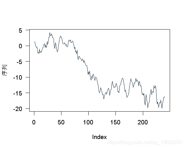
- Dickey Fuller(标准)
这里,对于Dickey-Fuller测试的简单版本,我们假设
我们想测试是否(或不是)。我们可以将以前的表示写为
所以我们只需测试线性回归中的回归系数是否为空。这可以通过学生t检验来完成。如果我们考虑前面的模型没有线性漂移,我们必须考虑下面的回归

 Call:
lm(formula = z.diff ~ 0 + z.lag.1)

Residuals:
     Min       1Q   Median       3Q      Max
-2.84466 -0.55723 -0.00494  0.63816  2.54352

Coefficients:
         Estimate Std. Error t value Pr(>|t|)
z.lag.1 -0.005609   0.007319  -0.766    0.444

Residual standard error: 0.963 on 238 degrees of freedom
Multiple R-squared:  0.002461,    Adjusted R-squared:  -0.00173
F-statistic: 0.5873 on 1 and 238 DF,  p-value: 0.4442
我们的测试程序将基于学生t检验的值,
> summary(lm(z.diff~0+z.lag.1 ))$coefficients[1,3]
[1] -0.7663308
这正是计算使用的值
ur.df(X,type="none",lags=0)


###############################################################
# Augmented Dickey-Fuller Test Unit Root / Cointegration Test #
###############################################################

The value of the test statistic is: -0.7663
可以使用临界值(99%、95%、90%)来解释该值
> qnorm(c(.01,.05,.1)/2)
[1] -2.575829 -1.959964 -1.644854
如果统计量超过这些值,那么序列就不是平稳的,因为我们不能拒绝这样的假设。所以我们可以得出结论,有一个单位根。实际上,这些临界值是通过
 ###############################################
# Augmented Dickey-Fuller Test Unit Root Test #
###############################################

Test regression none

Call:
lm(formula = z.diff ~ z.lag.1 - 1)

Residuals:
     Min       1Q   Median       3Q      Max
-2.84466 -0.55723 -0.00494  0.63816  2.54352

Coefficients:
         Estimate Std. Error t value Pr(>|t|)
z.lag.1 -0.005609   0.007319  -0.766    0.444

Residual standard error: 0.963 on 238 degrees of freedom
Multiple R-squared:  0.002461,    Adjusted R-squared:  -0.00173
F-statistic: 0.5873 on 1 and 238 DF,  p-value: 0.4442

Value of test-statistic is: -0.7663

Critical values for test statistics:
      1pct  5pct 10pct
tau1 -2.58 -1.95 -1.62
R有几个包可以用于单位根测试。
 Augmented Dickey-Fuller Test

data:  X
Dickey-Fuller = -2.0433, Lag order = 0, p-value = 0.5576
alternative hypothesis: stationary
这里还有一个检验零假设是存在单位根。但是p值是完全不同的。
随时关注您喜欢的主题
p.value
[1] 0.4423705
testreg$coefficients[4]
[1] 0.4442389- 增广Dickey-Fuller检验
回归中可能有一些滞后现象。例如,我们可以考虑
同样,我们需要检查一个系数是否为零。这可以用学生t检验来做。
 > summary(lm(z.diff~0+z.lag.1+z.diff.lag ))

Call:
lm(formula = z.diff ~ 0 + z.lag.1 + z.diff.lag)

Residuals:
     Min       1Q   Median       3Q      Max
-2.87492 -0.53977 -0.00688  0.64481  2.47556

Coefficients:
            Estimate Std. Error t value Pr(>|t|)
z.lag.1    -0.005394   0.007361  -0.733    0.464
z.diff.lag -0.028972   0.065113  -0.445    0.657

Residual standard error: 0.9666 on 236 degrees of freedom
Multiple R-squared:  0.003292,    Adjusted R-squared:  -0.005155
F-statistic: 0.3898 on 2 and 236 DF,  p-value: 0.6777

coefficients[1,3]
[1] -0.7328138
该值是使用
> df=ur.df(X,type="none",lags=1)

###############################################
# Augmented Dickey-Fuller Test Unit Root Test #
###############################################

Test regression none

Call:
lm(formula = z.diff ~ z.lag.1 - 1 + z.diff.lag)

Residuals:
     Min       1Q   Median       3Q      Max
-2.87492 -0.53977 -0.00688  0.64481  2.47556

Coefficients:
            Estimate Std. Error t value Pr(>|t|)
z.lag.1    -0.005394   0.007361  -0.733    0.464
z.diff.lag -0.028972   0.065113  -0.445    0.657

Residual standard error: 0.9666 on 236 degrees of freedom
Multiple R-squared:  0.003292,    Adjusted R-squared:  -0.005155
F-statistic: 0.3898 on 2 and 236 DF,  p-value: 0.6777

Value of test-statistic is: -0.7328

Critical values for test statistics:
      1pct  5pct 10pct
tau1 -2.58 -1.95 -1.62
同样,也可以使用其他包:
 Augmented Dickey-Fuller Test

data:  X
Dickey-Fuller = -1.9828, Lag order = 1, p-value = 0.5831
alternative hypothesis: stationary
结论是一样的(我们应该拒绝序列是平稳的假设)。
- 带趋势和漂移的增广Dickey-Fuller检验
到目前为止,我们的模型中还没有包括漂移。但很简单(这将被称为前一过程的扩充版本):我们只需要在回归中包含一个常数,
> summary(lm)


Residuals:
     Min       1Q   Median       3Q      Max
-2.91930 -0.56731 -0.00548  0.62932  2.45178

Coefficients:
            Estimate Std. Error t value Pr(>|t|)
(Intercept)  0.29175    0.13153   2.218   0.0275 *
z.lag.1     -0.03559    0.01545  -2.304   0.0221 *
z.diff.lag  -0.01976    0.06471  -0.305   0.7603
---
Signif. codes:  0 ‘***’ 0.001 ‘**’ 0.01 ‘*’ 0.05 ‘.’ 0.1 ‘ ’ 1

Residual standard error: 0.9586 on 235 degrees of freedom
Multiple R-squared:  0.02313,    Adjusted R-squared:  0.01482
F-statistic: 2.782 on 2 and 235 DF,  p-value: 0.06393
考虑到方差输出的一些分析,这里获得了感兴趣的统计数据,其中该模型与没有集成部分的模型进行了比较,以及漂移,
> summary(lmcoefficients[2,3]
[1] -2.303948
> anova(lm$F[2]
[1] 2.732912
这两个值也是通过
ur.df(X,type="drift",lags=1)

###############################################
# Augmented Dickey-Fuller Test Unit Root Test #
###############################################

Test regression drift

Residuals:
     Min       1Q   Median       3Q      Max
-2.91930 -0.56731 -0.00548  0.62932  2.45178

Coefficients:
            Estimate Std. Error t value Pr(>|t|)
(Intercept)  0.29175    0.13153   2.218   0.0275 *
z.lag.1     -0.03559    0.01545  -2.304   0.0221 *
z.diff.lag  -0.01976    0.06471  -0.305   0.7603
---
Signif. codes:  0 ‘***’ 0.001 ‘**’ 0.01 ‘*’ 0.05 ‘.’ 0.1 ‘ ’ 1

Residual standard error: 0.9586 on 235 degrees of freedom
Multiple R-squared:  0.02313,    Adjusted R-squared:  0.01482
F-statistic: 2.782 on 2 and 235 DF,  p-value: 0.06393

Value of test-statistic is: -2.3039 2.7329

Critical values for test statistics:
      1pct  5pct 10pct
tau2 -3.46 -2.88 -2.57
phi1  6.52  4.63  3.81
我们还可以包括一个线性趋势,
> temps=(lags+1):n
lm(z.diff~1+temps+z.lag.1+z.diff.lag )

Residuals:
     Min       1Q   Median       3Q      Max
-2.87727 -0.58802 -0.00175  0.60359  2.47789

Coefficients:
              Estimate Std. Error t value Pr(>|t|)
(Intercept)  0.3227245  0.1502083   2.149   0.0327 *
temps       -0.0004194  0.0009767  -0.429   0.6680
z.lag.1     -0.0329780  0.0166319  -1.983   0.0486 *
z.diff.lag  -0.0230547  0.0652767  -0.353   0.7243
---
Signif. codes:  0 ‘***’ 0.001 ‘**’ 0.01 ‘*’ 0.05 ‘.’ 0.1 ‘ ’ 1

Residual standard error: 0.9603 on 234 degrees of freedom
Multiple R-squared:  0.0239,    Adjusted R-squared:  0.01139
F-statistic:  1.91 on 3 and 234 DF,  p-value: 0.1287

> summary(lmcoefficients[3,3]
[1] -1.98282
> anova(lm$F[2]
[1] 2.737086
而R函数返回
ur.df(X,type="trend",lags=1)


###############################################
# Augmented Dickey-Fuller Test Unit Root Test #
###############################################

Test regression trend


Residuals:
     Min       1Q   Median       3Q      Max
-2.87727 -0.58802 -0.00175  0.60359  2.47789

Coefficients:
              Estimate Std. Error t value Pr(>|t|)
(Intercept)  0.3227245  0.1502083   2.149   0.0327 *
z.lag.1     -0.0329780  0.0166319  -1.983   0.0486 *
tt          -0.0004194  0.0009767  -0.429   0.6680
z.diff.lag  -0.0230547  0.0652767  -0.353   0.7243
---
Signif. codes:  0 ‘***’ 0.001 ‘**’ 0.01 ‘*’ 0.05 ‘.’ 0.1 ‘ ’ 1

Residual standard error: 0.9603 on 234 degrees of freedom
Multiple R-squared:  0.0239,    Adjusted R-squared:  0.01139
F-statistic:  1.91 on 3 and 234 DF,  p-value: 0.1287

Value of test-statistic is: -1.9828 1.8771 2.7371

Critical values for test statistics:
      1pct  5pct 10pct
tau3 -3.99 -3.43 -3.13
phi2  6.22  4.75  4.07
phi3 8.43 6.49 5.47- KPSS 检验
在这里,在KPSS过程中,可以考虑两种模型:漂移模型或线性趋势模型。在这里,零假设是序列是平稳的。
代码是
ur.kpss(X,type="mu")

#######################
# KPSS Unit Root Test #
#######################

Test is of type: mu with 4 lags.

Value of test-statistic is: 0.972

Critical value for a significance level of:
                10pct  5pct 2.5pct  1pct
critical values 0.347 0.463  0.574 0.73
在这种情况下,有一种趋势
ur.kpss(X,type="tau")

#######################
# KPSS Unit Root Test #
#######################

Test is of type: tau with 4 lags.

Value of test-statistic is: 0.5057

Critical value for a significance level of:
                10pct  5pct 2.5pct  1pct
critical values 0.119 0.146  0.176 0.216
再一次,可以使用另一个包来获得相同的检验(但同样,不同的输出)
 KPSS Test for Level Stationarity

data:  X
KPSS Level = 1.1997, Truncation lag parameter = 3, p-value = 0.01

> kpss.test(X,"Trend")

    KPSS Test for Trend Stationarity

data:  X
KPSS Trend = 0.6234, Truncation lag parameter = 3, p-value = 0.01
至少有一致性,因为我们一直拒绝假设。
- Philipps-Perron 检验
Philipps-Perron检验基于ADF过程。代码
> PP.test(X)

    Phillips-Perron Unit Root Test

data:  X
Dickey-Fuller = -2.0116, Truncation lag parameter = 4, p-value = 0.571
另一种可能的替代方案是
> pp.test(X)

    Phillips-Perron Unit Root Test

data:  X
Dickey-Fuller Z(alpha) = -7.7345, Truncation lag parameter = 4, p-value
= 0.6757
alternative hypothesis: stationary- 比较
我不会花更多的时间比较不同的代码,在R中,运行这些测试。我们再花点时间快速比较一下这三种方法。让我们生成一些或多或少具有自相关的自回归过程,以及一些随机游走,让我们看看这些检验是如何执行的:
 > for(i in 1:(length(AR)+1)
+ for(s in 1:1000){
+ if(i!=1) X=arima.sim
+ M2[s,i]=(pp.testp.value)
+ M1[s,i]=(kpss.testp.value)
+ M3[s,i]=(adf.testp.value)
+ }
这里,我们要计算检验的p值超过5%的次数,
 > plot(AR,P[1,],type="l",col="red",ylim=c(0,1)
> lines(AR,P[2,],type="l",col="blue")
> lines(AR,P[3,],type="l",col="green")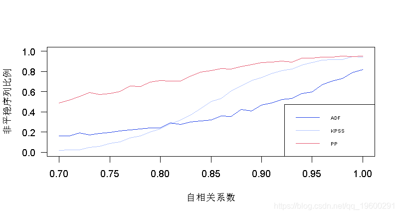
我们可以在这里看到Dickey-Fuller测试的表现有多不稳定,因为我们的自回归过程中有50%(至少)被认为是非平稳的。
 Python实现Transformer神经网络时间序列模型可视化分析商超蔬菜销售数据筛选高销量单品预测|附代码数据
 Python对2028奥运奖牌预测分析:贝叶斯推断、梯度提升机GBM、时间序列、随机森林、二元分类教练效应量化研究
 Python用Transformer、SARIMAX、RNN、LSTM、Prophet时间序列预测对比分析用电量、零售销售、公共安全、交通事故数据
 Python比特币价格时间序列:LGBMRegressor递归自回归、随机游走及外部变量预测探索