In order to find out the main factors affecting price fluctuations, we use stepwise regression to eliminate some independent variables that have little impact on the dependent variable, that is, the price. The name of the variable is changed to x1, x2…
The last emergency event needs to use dummy variables. Only two dummy variables are needed. We will use them as the three parameters X49, X50, X51, and set their values to “positive” “Effect”, “No effect”, and “Negative effect” were changed to -1,0,1.
可下载资源
We respectively changed the names of independent variables such as WTI Price Field Production of Crude Oil (Thousand Barrels) to x1, x2… The last emergency event needs to use dummy variables. Only two dummy variables are needed, we will use them as X49, X50, X51, three parameters and their values ”positive influence”, “no influence”, “negative influence” were changed to -1,0,1.
rugarch
This has the idea of a specification for a model that is a separate object. Then there are functions for fitting (that is, estimating parameters), predicting and simulation.
Here is an example of fitting with a Student t distribution:
The optimization in this package is perhaps the most sophisticated and trustworthy among the packages that I discuss.
fGarch
We’ll fit the same Student t model as above:
tseries
I believe that this package was the first to include a publicly available garch function in R. It is restricted to the normal distribution.
bayesGARCH
I think Bayes estimation of garch models is a very natural thing to do. We have fairly specific knowledge about what the parameter values should look like.
The only model this package does is the garch(1,1) with t distributed errors. So we are happy in that respect.
However, this command fails with an error. The default is to use essentially uninformative priors — presumably this problem demands some information. In practice we would probably want to give it informative priors anyway.
betategarch
This package fits an EGARCH model with t distributed errors. EGARCH is a clever model that makes some things easier and other things harder.
That the plotting function is
After R language processing, we get the model
Y~x1 + x2 + x4 + x5 + x7 + x13 + x14 + x15 + x16 + x17 + x18 + x20 + x21 + x23 + x34 + x25 + x26 + x29 + x30 + x33 + x35 + x36 + x37 + x39 + x40 + x42 + x44 + x46 + x47 + x48 + x49 + x50
It can be seen that those with less impact have been eliminated.
Garch model predicts volatility
We use the Garch model to predict volatility,

First check the normality of the data, you can calculate the data distribution function, QQ chart, logarithmic return rate series line chart

> shapiro.test(rlogdiffdata)

	Shapiro-Wilk normality test

data:  rlogdiffdata
W = 0.94315, p-value = 1.458e-05
It can be seen from the QQ graph and the p-value that the data roughly conforms to the normal distribution.
Finally, use the VaR curve to warn of severe fluctuations.
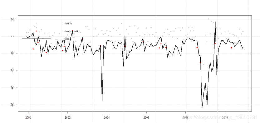
The red points are the warning points before severe fluctuations.
Strong impact point analysis
We can find strong influence points by using cook statistics, so we use the influence.measures() function of R language for influence analysis.
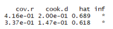
The ones with * on the right represent strong influence points.
We construct the F test through the studentized residuals, and finally get the t test to detect abnormal points. by
stdres<-rstudent(lm.sol)To get the studentized residual, and then use the formula
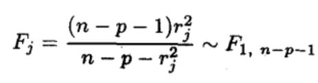
To calculate Fj and finally convert it to tj,
t=sqrt((144-51-1)*stdres^2/(144-51-stdres^2))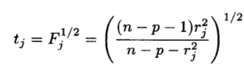
Finally we can check if![]() Then it is an abnormal point.
Then it is an abnormal point.
R language execution
res<-t>abs(qt(.025, df=92)) You can directly get a Boolean value greater than the corresponding t value.
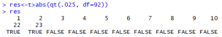
A value of True may be an abnormal point.
prediction
We used HoltWinters to predict our oil price range
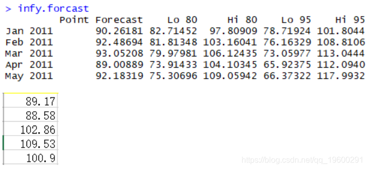
The true value is basically within the predicted range, but it is still more difficult to predict the net profit.
可下载资源
关于作者
Kaizong Ye是拓端研究室(TRL)的研究员。在此对他对本文所作的贡献表示诚挚感谢,他在上海财经大学完成了统计学专业的硕士学位,专注人工智能领域。擅长Python.Matlab仿真、视觉处理、神经网络、数据分析。
本文借鉴了作者最近为《R语言数据分析挖掘必知必会 》课堂做的准备。
非常感谢您阅读本文,如需帮助请联系我们!
 视频讲解|Stata和R语言自助法Bootstrap结合GARCH对sp500收益率数据分析
 R语言股价跳跃点识别:隐马尔可夫hmm和GARCH-Jump对sp500金融时间序列分析
 【视频讲解】Python用LSTM长短期记忆网络GARCH对SPX指数金融时间序列波动率滚动预测
 R 语言GJR-GARCH、GARCH-t、GARCH-ged分析金融时间序列数据波动性预测、检验、可视化