包含更多的预测变量不是免费的：在系数估算的更多可变性，更难的解释以及可能包含高度依赖的预测变量方面要付出代价。

由Kaizong Ye，Coin Ge撰写

确实，对于样本大小

，在线性模型中可以考虑 的预测变量最大数量为 p 。或等效地，使用预测变量p 拟合模型需要最小样本量

。

可下载资源

完整程序、数据和文档（word）

如果我们考虑p = 1 和 p = 2 的几何，这一事实的解释很简单：

如果p = 1，则至少需要n = 2个点才能唯一地拟合一条线。但是，这条线没有给出关于其周围变化的信息，因此无法估计。因此，我们至少需要个点，换句话说就是。
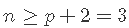如果p = 2 ，则至少需要n = 3个点才能唯一地拟合平面。但是同样，该平面没有提供有关其周围数据变化的信息，因此无法估计。因此，我们需要。

逐步回归主要解决的是多变量共线性问题，也就是 $x_{1},x_{2},..,x_{m}$ 不是线性无关的关系，它是基于变量解释性来进行特征提取的一种回归方法。

逐步回归的主要做法有三种：

（一）Forward selection：将自变量逐个引入模型，引入一个自变量后要查看该变量的引入是否使得模型发生显著性变化（F检验），如果发生了显著性变化，那么则将该变量引入模型中，否则忽略该变量，直至所有变量都进行了考虑。即将变量按照贡献度从大到小排列，依次加入。

步骤：

（1）建立每个自变量与因变量的一元回归方程： $y=a_{i}X_{i}+b_{i},i=1,2,..,m$

（2）分别计算m个一元回归方程中的回归系数的检验统计量F，并求出最大值为 $F_{k_{1}}^{1}=\max \left\{F_{1}^{1}, F_{2}^{1}, \cdots, F_{m}^{1}\right\}$ ，

若 $F_{k_{1}}^{1} \leq F_{\alpha}(1, n-2)$ ，停止筛选，否则将 $x_{k_{1}}$ 选入变量集，此时可以将 $x_{k_{1}}$ 看做 $x_{1}$ ，进入步骤（3）

（3）分别将自变量组 $(x_{1},x_{2}),(x_{1},x_{3}),...,(x_{1},x_{m})$ 与因变量建立二元回归方程，（此时 $x_{1}$ 是步骤2中的 $x_{k_{1}}$ ）计算方程中 $x_{2},x_{3},..,x_{m}$ 的回归系数检验统计量F，取 $F_{k_{2}}^{2}=\max \left\{F_{2}^{2}, F_{3}^{2}, \cdots, F_{m}^{2}\right\}$ ，若 $F_{k_{2}}^{2} \leq F_{\alpha}(1, n-2-1)$ 则停止筛选，否则将 $x_{k_{2}}$ 选入变量集，此时将 $x_{k_{2}}$ 看做 $x_{2}$ ….如此迭代直到自变量的最大的F值小于临界值，此时回归方程就是最优的回归方程。

特点：自变量一旦选入，则永远保存在模型中；不能反映自变量选进模型后的模型本身的变化情况。

（2）Backward elimination：与Forward selection选择相反，在这个方法中，将所有变量放入模型，然后尝试将某一变量进行剔除，查看剔除后对整个模型是否有显著性变化（F检验），如果没有显著性变化则剔除，若有则保留，直到留下所有对模型有显著性变化的因素。即将自变量按贡献度从小到大，依次剔除。

步骤：

（1）建立全部 $x_{1},x_{2},..,x_{m}$ 对因变量y的回归方程，对方程中的m个自变量进行F检验，取最小值为： $F_{k_{1}}^{1}=\min \left\{F_{1}^{1}, F_{2}^{1}, \cdots, F_{m}^{1}\right\}$ ，若 $F_{k_{1}}^{1}>F_{\alpha}(1, n-m-1)” class=”mathcode” src=”https://private.codecogs.com/gif.latex?F_%7Bk_%7B1%7D%7D%5E%7B1%7D%3EF_%7B%5Calpha%7D%281%2C%20n-m-1%29″ style=”outline: none; border: 0px; cursor: zoom-in;”>，则没有自变量可剔除，此时回归方程就是最优的；否则剔除<img decoding=$ ，在此时可另 $x_{k_{1}}$ 为 $x_{m}$ ，进入步骤（2）

（2）建立 $x_{1},x_{2},..,x_{m-1}$ 与因变量y的回归方程，对方程中的回归系数进行F检验，取最小值 $F_{k_{2}}^{2}=\min \left\{F_{1}^{2}, F_{2}^{2}, \cdots, F_{m-1}^{2}\right\}$ ，若 $F_{k_{2}}^{2}>F_{\alpha}(1, n-(m-1)-1)” class=”mathcode” src=”https://private.codecogs.com/gif.latex?F_%7Bk_%7B2%7D%7D%5E%7B2%7D%3EF_%7B%5Calpha%7D%281%2C%20n-%28m-1%29-1%29″ style=”outline: none; border: 0px; cursor: zoom-in;”>，则无变量需要剔除，此时方程就是最优的，否则将<img decoding=$ 剔除，此时设 $x_{k_{2}}$ 为 $x_{m-1}$ ，…,一直迭代下去，直到各变量的回归系数F值均大于临界值，即方程中没有变量可以剔除为止，此时的回归方程就是最优的回归方程。

特点：自变量一旦剔除，则不再进入模型；开始把全部自变量引入模型，计算量过大。

（3）Bidirectional elimination：逐步筛选法。是在第一个的基础上做一定的改进，当引入一个变量后，首先查看这个变量是否使得模型发生显著性变化（F检验），若发生显著性变化，再对所有变量进行t检验，当原来引入变量由于后面加入的变量的引入而不再显著变化时，则剔除此变量，确保每次引入新的变量之前回归方程中只包含显著性变量，直到既没有显著的解释变量选入回归方程，也没有不显著的解释变量从回归方程中剔除为止，最终得到一个最优的变量集合。

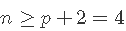下一部分代码的输出阐明了和之间的区别。

假设数据：n个观测值，p = n-1个预测变量。


 
n <- 5
p <- n - 1
df <- data.frame(y = rnorm(n), x = matrix(rnorm(n * p), nrow = n, ncol = p))
 
# 情况p = n-1 = 2：可以估计beta，但不能估计sigma ^ 2（因此，不能执行推断，因为它需要估计的sigma ^ 2）
 
 
summary(lm(y ~ ., data = df))
 
# 情况p = n-2 = 1：可以估计beta和sigma ^ 2（因此可以进行推断）
 
summary(lm(y ~ . - x.1, data = df))

课程

R语言数据分析挖掘必知必会

从数据获取和清理开始，有目的的进行探索性分析与可视化。让数据从生涩的资料，摇身成为有温度的故事。

立即参加 ➜

当减小时，自由度量化的变异性的增加。

既然我们已经更多地了解了预测变量过多的问题，我们将重点放在为多元回归模型选择最合适的预测变量上。如果没有独特的解决方案，这将是一项艰巨的任务。但是，有一个行之有效的程序通常会产生良好的结果： 逐步模型选择。其原理是依次比较具有不同预测变量的多个线性回归模型。

在介绍该方法之前，我们需要了解什么是 信息准则。信息标准在模型的适用性与采用的预测变量数量之间取得平衡。两个常见标准是 贝叶斯信息标准 （BIC）和 赤池信息标准 （AIC）。两者都基于 模型适用性和复杂性之间的平衡：

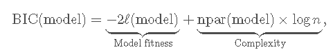
其中是模型的对 数似然度 （模型拟合数据的程度），而是考虑的参数数量在模型中，对于具有p个预测变量的多元线性回归模型，则为p + 2。AIC在用替换了，因此，与BIC相比，它对 较复杂的模型的处罚较少。这就是为什么一些从业者更喜欢BIC进行模型比较的原因之一。BIC和AIC可以通过BIC 和计算 AIC。

我们使用地区房价数据，变量介绍：

（1）town：每一个人口普查区所在的城镇

（2）LON: 人口普查区中心的经度

（3）LAT: 人口普查区中心的纬度

（4）MEDV: 每一个人口普查区所对应的房子价值的中位数 (单位为$1000)

（5）CRIM: 人均犯罪率

（6）ZN: 土地中有多少是地区是大量住宅物业

（7）INDUS: 区域中用作工业用途的土地占比

（8）CHAS: 1：该人口普查区紧邻查尔斯河；0：该人口普查区没有紧邻查尔斯河

（9）NOX: 空气中氮氧化物的集中度 (衡量空气污染的指标)

（10）RM: 每个房子的平均房间数目

（11）AGE: 建于1940年以前的房子的比例

（12）DIS: 该人口普查区距离波士顿市中心的距离

（13）RAD: 距离重要高速路的远近程度 (1代表最近；24代表最远)

（14）TAX: 房子每$10,000价值所对应的税收金额

（15）PTRATIO: 该城镇学生与老师的比例

最受欢迎的见解

1.R语言多元Logistic逻辑回归应用案例

2.面板平滑转移回归(PSTR)分析案例实现

3.matlab中的偏最小二乘回归（PLSR）和主成分回归（PCR）

4.R语言泊松Poisson回归模型分析案例

5.R语言回归中的Hosmer-Lemeshow拟合优度检验

6.r语言中对LASSO回归，Ridge岭回归和Elastic Net模型实现

7.在R语言中实现Logistic逻辑回归

8.python用线性回归预测股票价格

9.R语言如何在生存分析与Cox回归中计算IDI，NRI指标

他们将作为模型输入。

# 具有不同预测变量的两个模型
 
mod1 <- lm(medv ~ age + crim, data = Boston)
mod2 <- lm(medv ~ age + crim + lstat, data = Boston)
# BICs
BIC(mod1)
## [1] 3581.893
BIC(mod2) # 较小->较好
## [1] 3300.841
# AICs
AIC(mod1)
## [1] 3564.987
AIC(mod2) # 较小->较好
## [1] 3279.708
# 检查摘要
 
## 
## Residuals:
##     Min      1Q  Median      3Q     Max 
## -13.940  -4.991  -2.420   2.110  32.033 
## 
## Coefficients:
##             Estimate Std. Error t value Pr(>|t|)    
## (Intercept) 29.80067    0.97078  30.698  < 2e-16 ***
## age         -0.08955    0.01378  -6.499 1.95e-10 ***
## crim        -0.31182    0.04510  -6.914 1.43e-11 ***
## ---
## Signif. codes:  0 '***' 0.001 '**' 0.01 '*' 0.05 '.' 0.1 ' ' 1
## 
## Residual standard error: 8.157 on 503 degrees of freedom
## Multiple R-squared:  0.2166, Adjusted R-squared:  0.2134 
## F-statistic: 69.52 on 2 and 503 DF,  p-value: < 2.2e-16
summary(mod2)
## 
## Call:
## lm(formula = medv ~ age + crim + lstat, data = Boston)
## 
## Residuals:
##     Min      1Q  Median      3Q     Max 
## -16.133  -3.848  -1.380   1.970  23.644 
## 
## Coefficients:
##             Estimate Std. Error t value Pr(>|t|)    
## (Intercept) 32.82804    0.74774  43.903  < 2e-16 ***
## age          0.03765    0.01225   3.074  0.00223 ** 
## crim        -0.08262    0.03594  -2.299  0.02193 *  
## lstat       -0.99409    0.05075 -19.587  < 2e-16 ***
## ---
## Signif. codes:  0 '***' 0.001 '**' 0.01 '*' 0.05 '.' 0.1 ' ' 1
## 
## Residual standard error: 6.147 on 502 degrees of freedom
## Multiple R-squared:  0.5559, Adjusted R-squared:  0.5533 
## F-statistic: 209.5 on 3 and 502 DF,  p-value: < 2.2e-16

让我们回到预测变量的选择。如果我们有p个预测变量，那么一个简单的过程就是检查所有可用它们构建的可能模型，然后根据BIC / AIC选择最佳模型。这就是所谓的 最佳子集选择。问题在于存在个可能的模型！
让我们看看如何研究 wine 数据集，将使用所有可用预测变量的数据作为初始模型。

R语言逐步多元回归模型分析长鼻鱼密度影响因素

阅读文章 ➜

波尔多是法国的葡萄酒产区。尽管这种酒的生产方式几乎相同，但已有数百年历史，但每年的价格和质量差异有时非常显着。人们普遍认为波尔多葡萄酒陈年越老越好，因此有动力去储存葡萄酒直至成熟。主要问题在于，仅通过品尝就很难确定葡萄酒的质量，因为在实际饮用时，味道会发生很大变化。这就是为什么葡萄酒品尝师和专家会有所帮助的原因。他们品尝葡萄酒，然后预测以后将是最好的葡萄酒。
1990年3月4日，《纽约时报》宣布普林斯顿大学经济学教授奥利·阿森费尔特（Orley Ashenfelter）可以预测波尔多葡萄酒的质量而无需品尝一滴。 Ashenfelter使用了一种称为线性回归的方法。该方法预测结果变量或因变量。作为自变量，他使用了酒的年份（因此，较老的酒会更昂贵）和与天气有关的信息，特别是平均生长季节温度，收成雨和冬雨。

stepAIC 将参数 k 设为2 （默认值）或，其中n是样本大小。k = 2 它采用AIC准则， k = log(n) 它采用BIC准则。


# 完整模型
 
# 用 BIC
## Start:  AIC=-53.29
## Price ~ Year + WinterRain + AGST + HarvestRain + Age + FrancePop
## 
## 
## Step:  AIC=-53.29
## Price ~ Year + WinterRain + AGST + HarvestRain + FrancePop
## 
##               Df Sum of Sq    RSS     AIC
## - FrancePop    1    0.0026 1.8058 -56.551
## - Year         1    0.0048 1.8080 -56.519
## <none>                     1.8032 -53.295
## - WinterRain   1    0.4585 2.2617 -50.473
## - HarvestRain  1    1.8063 3.6095 -37.852
## - AGST         1    3.3756 5.1788 -28.105
## 
## Step:  AIC=-56.55
## Price ~ Year + WinterRain + AGST + HarvestRain
## 
##               Df Sum of Sq    RSS     AIC
## <none>                     1.8058 -56.551
## - WinterRain   1    0.4809 2.2867 -53.473
## - Year         1    0.9089 2.7147 -48.840
## - HarvestRain  1    1.8760 3.6818 -40.612
## - AGST         1    3.4428 5.2486 -31.039
 
summary(modBIC)
## 
## Call:
## lm(formula = Price ~ Year + WinterRain + AGST + HarvestRain, 
##     data = wine)
## 
## Residuals:
##      Min       1Q   Median       3Q      Max 
## -0.46024 -0.23862  0.01347  0.18601  0.53443 
## 
## Coefficients:
##               Estimate Std. Error t value Pr(>|t|)    
## (Intercept) 43.6390418 14.6939240   2.970  0.00707 ** 
## Year        -0.0238480  0.0071667  -3.328  0.00305 ** 
## WinterRain   0.0011667  0.0004820   2.420  0.02421 *  
## AGST         0.6163916  0.0951747   6.476 1.63e-06 ***
## HarvestRain -0.0038606  0.0008075  -4.781 8.97e-05 ***
## ---
## Signif. codes:  0 '***' 0.001 '**' 0.01 '*' 0.05 '.' 0.1 ' ' 1
## 
## Residual standard error: 0.2865 on 22 degrees of freedom
## Multiple R-squared:  0.8275, Adjusted R-squared:  0.7962 
## F-statistic: 26.39 on 4 and 22 DF,  p-value: 4.057e-08
# 用 AIC
## Start:  AIC=-61.07
## Price ~ Year + WinterRain + AGST + HarvestRain + Age + FrancePop
## 
## 
## Step:  AIC=-61.07
## Price ~ Year + WinterRain + AGST + HarvestRain + FrancePop
## 
##               Df Sum of Sq    RSS     AIC
## - FrancePop    1    0.0026 1.8058 -63.031
## - Year         1    0.0048 1.8080 -62.998
## <none>                     1.8032 -61.070
## - WinterRain   1    0.4585 2.2617 -56.952
## - HarvestRain  1    1.8063 3.6095 -44.331
## - AGST         1    3.3756 5.1788 -34.584
## 
## Step:  AIC=-63.03
## Price ~ Year + WinterRain + AGST + HarvestRain
## 
##               Df Sum of Sq    RSS     AIC
## <none>                     1.8058 -63.031
## - WinterRain   1    0.4809 2.2867 -58.656
## - Year         1    0.9089 2.7147 -54.023
## - HarvestRain  1    1.8760 3.6818 -45.796
## - AGST         1    3.4428 5.2486 -36.222
summary(modAIC)
## 
## Call:
## lm(formula = Price ~ Year + WinterRain + AGST + HarvestRain, 
##     data = wine)
## 
## Residuals:
##      Min       1Q   Median       3Q      Max 
## -0.46024 -0.23862  0.01347  0.18601  0.53443 
## 
## Coefficients:
##               Estimate Std. Error t value Pr(>|t|)    
## (Intercept) 43.6390418 14.6939240   2.970  0.00707 ** 
## Year        -0.0238480  0.0071667  -3.328  0.00305 ** 
## WinterRain   0.0011667  0.0004820   2.420  0.02421 *  
## AGST         0.6163916  0.0951747   6.476 1.63e-06 ***
## HarvestRain -0.0038606  0.0008075  -4.781 8.97e-05 ***
## ---
## Signif. codes:  0 '***' 0.001 '**' 0.01 '*' 0.05 '.' 0.1 ' ' 1
## 
## Residual standard error: 0.2865 on 22 degrees of freedom
## Multiple R-squared:  0.8275, Adjusted R-squared:  0.7962 
## F-statistic: 26.39 on 4 and 22 DF,  p-value: 4.057e-08

接下来是stepAIC 对执行情况的解释。在每个步骤中， stepAIC 显示有关信息标准当前值的信息。例如，对于 modBIC，第一步的BIC是Step: AIC=-53.29 ，然后在第二步进行了改进 Step: AIC=-56.55 （即使使用“ BIC”，该功能也会始终输出“ AIC”）。下一个继续前进的模型是stepAIC 通过研究添加或删除预测变量后得出的不同模型的信息标准来决定的（取决于 direction 参数，在下文中进行解释）。例如modBIC在第一步中，删除导致的模型 FrancePop 的BIC等于 -56.551，如果 Year 删除，则BIC将为 -56.519。逐步回归，然后删除 FrancePop （因为它给出了最低的BIC），然后重复此过程，最终导致删除 <none> 预测变量是可能的最佳操作。下面的代码块说明了stepsAIC的输出 extractAIC，和BIC / AIC的输出BIC/ AIC。

# 相同的BIC，标准不同
 
 
AIC(modBIC, k = log(n))
## [1] -56.55135
BIC(modBIC)
## [1] 23.36717
# 观察到MASS :: stepAIC（mod，k = log（nrow（wine）））返回的最终BIC是由extractAIC（）而不是BIC（）给出的！但是两者是等效的 
# 相同的AIC，标准不同
 
 
AIC(modBIC, k = 2)
## [1] -63.03053
BIC(modBIC)
## [1] 23.36717
 
 
BIC(modBIC) - AIC(modBIC
## [1] 79.91852
n * (log(2 * pi+ 1) + log(n)
## [1] 79.91852
#与AIC相同
 
 
AIC(modAIC) - AIC(modAIC
## [1] 78.62268
n * (log(2 * pi + 1 + 2
## [1] 78.62268

随时关注您喜欢的主题

# 相同的BIC，标准不同
 
 
AIC(modBIC, k = log(n))
## [1] -56.55135
BIC(modBIC)
## [1] 23.36717
# 观察到MASS :: stepAIC（mod，k = log（nrow（wine）））返回的最终BIC是由extractAIC（）而不是BIC（）给出的！但是两者是等效的 
# 相同的AIC，标准不同
 
 
AIC(modBIC, k = 2)
## [1] -63.03053
BIC(modBIC)
## [1] 23.36717
 
 
BIC(modBIC) - AIC(modBIC
## [1] 79.91852
n * (log(2 * pi+ 1) + log(n)
## [1] 79.91852
#与AIC相同
 
 
AIC(modAIC) - AIC(modAIC
## [1] 78.62268
n * (log(2 * pi + 1 + 2
## [1] 78.62268


# 将无关的预测变量添加到葡萄酒数据集中
# 向后选择：从给定模型中顺序删除预测变量
 
# 从具有所有预测变量的模型开始
 
 
 
modAll, direction = "backward", k = log(n)
## Start:  AIC=-50.13
## Price ~ Year + WinterRain + AGST + HarvestRain + Age + FrancePop + 
##     noisePredictor
## 
## 
## Step:  AIC=-50.13
## Price ~ Year + WinterRain + AGST + HarvestRain + FrancePop + 
##     noisePredictor
## 
##                  Df Sum of Sq    RSS     AIC
## - FrancePop       1    0.0036 1.7977 -53.376
## - Year            1    0.0038 1.7979 -53.374
## - noisePredictor  1    0.0090 1.8032 -53.295
## <none>                        1.7941 -50.135
## - WinterRain      1    0.4598 2.2539 -47.271
## - HarvestRain     1    1.7666 3.5607 -34.923
## - AGST            1    3.3658 5.1599 -24.908
## 
## Step:  AIC=-53.38
## Price ~ Year + WinterRain + AGST + HarvestRain + noisePredictor
## 
##                  Df Sum of Sq    RSS     AIC
## - noisePredictor  1    0.0081 1.8058 -56.551
## <none>                        1.7977 -53.376
## - WinterRain      1    0.4771 2.2748 -50.317
## - Year            1    0.9162 2.7139 -45.552
## - HarvestRain     1    1.8449 3.6426 -37.606
## - AGST            1    3.4234 5.2212 -27.885
## 
## Step:  AIC=-56.55
## Price ~ Year + WinterRain + AGST + HarvestRain
## 
##               Df Sum of Sq    RSS     AIC
## <none>                     1.8058 -56.551
## - WinterRain   1    0.4809 2.2867 -53.473
## - Year         1    0.9089 2.7147 -48.840
## - HarvestRain  1    1.8760 3.6818 -40.612
## - AGST         1    3.4428 5.2486 -31.039
## 
## Call:
## lm(formula = Price ~ Year + WinterRain + AGST + HarvestRain, 
##     data = wineNoise)
## 
## Coefficients:
## (Intercept)         Year   WinterRain         AGST  HarvestRain  
##   43.639042    -0.023848     0.001167     0.616392    -0.003861
# 从中间模型开始
 
 
AIC(modInter, direction = "backward", k = log(n)
## Start:  AIC=-32.38
## Price ~ noisePredictor + Year + AGST
## 
##                  Df Sum of Sq    RSS     AIC
## - noisePredictor  1    0.0146 5.0082 -35.601
## <none>                        4.9936 -32.384
## - Year            1    0.7522 5.7459 -31.891
## - AGST            1    3.2211 8.2147 -22.240
## 
## Step:  AIC=-35.6
## Price ~ Year + AGST
## 
##        Df Sum of Sq    RSS     AIC
## <none>              5.0082 -35.601
## - Year  1    0.7966 5.8049 -34.911
## - AGST  1    3.2426 8.2509 -25.417
## 
## Call:
## lm(formula = Price ~ Year + AGST, data = wineNoise)
## 
## Coefficients:
## (Intercept)         Year         AGST  
##    41.49441     -0.02221      0.56067
# Recall that other predictors not included in modInter are not explored
# during the search (so the relevant predictor HarvestRain is not added)
# 正向选择：从给定模型顺序添加预测变量
 
# 从没有预测变量的模型开始，仅截距模型（表示为〜1）
 
 
AIC(modZero, direction = "forward"
## Start:  AIC=-22.28
## Price ~ 1
## 
##                  Df Sum of Sq     RSS     AIC
## + AGST            1    4.6655  5.8049 -34.911
## + HarvestRain     1    2.6933  7.7770 -27.014
## + FrancePop       1    2.4231  8.0472 -26.092
## + Year            1    2.2195  8.2509 -25.417
## + Age             1    2.2195  8.2509 -25.417
## <none>                        10.4703 -22.281
## + WinterRain      1    0.1905 10.2798 -19.481
## + noisePredictor  1    0.1761 10.2942 -19.443
## 
## Step:  AIC=-34.91
## Price ~ AGST
## 
##                  Df Sum of Sq    RSS     AIC
## + HarvestRain     1   2.50659 3.2983 -46.878
## + WinterRain      1   1.42392 4.3809 -39.214
## + FrancePop       1   0.90263 4.9022 -36.178
## + Year            1   0.79662 5.0082 -35.601
## + Age             1   0.79662 5.0082 -35.601
## <none>                        5.8049 -34.911
## + noisePredictor  1   0.05900 5.7459 -31.891
## 
## Step:  AIC=-46.88
## Price ~ AGST + HarvestRain
## 
##                  Df Sum of Sq    RSS     AIC
## + FrancePop       1   1.03572 2.2625 -53.759
## + Year            1   1.01159 2.2867 -53.473
## + Age             1   1.01159 2.2867 -53.473
## + WinterRain      1   0.58356 2.7147 -48.840
## <none>                        3.2983 -46.878
## + noisePredictor  1   0.06084 3.2374 -44.085
## 
## Step:  AIC=-53.76
## Price ~ AGST + HarvestRain + FrancePop
## 
##                  Df Sum of Sq    RSS     AIC
## + WinterRain      1   0.45456 1.8080 -56.519
## <none>                        2.2625 -53.759
## + noisePredictor  1   0.00829 2.2542 -50.562
## + Age             1   0.00085 2.2617 -50.473
## + Year            1   0.00085 2.2617 -50.473
## 
## Step:  AIC=-56.52
## Price ~ AGST + HarvestRain + FrancePop + WinterRain
## 
##                  Df Sum of Sq    RSS     AIC
## <none>                        1.8080 -56.519
## + noisePredictor  1 0.0100635 1.7979 -53.374
## + Year            1 0.0048039 1.8032 -53.295
## + Age             1 0.0048039 1.8032 -53.295
## 
## Call:
## lm(formula = Price ~ AGST + HarvestRain + FrancePop + WinterRain, 
##     data = wineNoise)
## 
## Coefficients:
## (Intercept)         AGST  HarvestRain    FrancePop   WinterRain  
##  -5.945e-01    6.127e-01   -3.804e-03   -5.189e-05    1.136e-03
# 在进行正向搜索时，充分设置范围参数非常重要！在范围中，您必须定义包含可探索模型集的“最小”（下部）和“最大”（上部）模型。如果未提供，则将最大模型用作传递的起始模型（在这种情况下为modZero），而stepAIC将不执行任何搜索
 
 
#从中间模型开始
 
 
## Start:  AIC=-32.38
## Price ~ noisePredictor + Year + AGST
## 
##               Df Sum of Sq    RSS     AIC
## + HarvestRain  1   2.71878 2.2748 -50.317
## + WinterRain   1   1.35102 3.6426 -37.606
## <none>                     4.9936 -32.384
## + FrancePop    1   0.24004 4.7536 -30.418
## 
## Step:  AIC=-50.32
## Price ~ noisePredictor + Year + AGST + HarvestRain
## 
##              Df Sum of Sq    RSS     AIC
## + WinterRain  1   0.47710 1.7977 -53.376
## <none>                    2.2748 -50.317
## + FrancePop   1   0.02094 2.2539 -47.271
## 
## Step:  AIC=-53.38
## Price ~ noisePredictor + Year + AGST + HarvestRain + WinterRain
## 
##             Df Sum of Sq    RSS     AIC
## <none>                   1.7977 -53.376
## + FrancePop  1 0.0036037 1.7941 -50.135
## 
## Call:
## lm(formula = Price ~ noisePredictor + Year + AGST + HarvestRain + 
##     WinterRain, data = wineNoise)
## 
## Coefficients:
##    (Intercept)  noisePredictor            Year            AGST     HarvestRain      WinterRain  
##      44.096639       -0.019617       -0.024126        0.620522       -0.003840        ＃回想一下，在搜索期间不会删除modInter中包含的预测变量（因此会保留无关的noisePredictor）
 
#两种选择：如果从中间模型开始，则很有用
 
#消除了与从中间模型完成的“向后”和“向前”搜索相关的问题
 
## Start:  AIC=-32.38
## Price ~ noisePredictor + Year + AGST
## 
##                  Df Sum of Sq    RSS     AIC
## + HarvestRain     1    2.7188 2.2748 -50.317
## + WinterRain      1    1.3510 3.6426 -37.606
## - noisePredictor  1    0.0146 5.0082 -35.601
## <none>                        4.9936 -32.384
## - Year            1    0.7522 5.7459 -31.891
## + FrancePop       1    0.2400 4.7536 -30.418
## - AGST            1    3.2211 8.2147 -22.240
## 
## Step:  AIC=-50.32
## Price ~ noisePredictor + Year + AGST + HarvestRain
## 
##                  Df Sum of Sq    RSS     AIC
## - noisePredictor  1   0.01182 2.2867 -53.473
## + WinterRain      1   0.47710 1.7977 -53.376
## <none>                        2.2748 -50.317
## + FrancePop       1   0.02094 2.2539 -47.271
## - Year            1   0.96258 3.2374 -44.085
## - HarvestRain     1   2.71878 4.9936 -32.384
## - AGST            1   2.94647 5.2213 -31.180
## 
## Step:  AIC=-53.47
## Price ~ Year + AGST + HarvestRain
## 
##                  Df Sum of Sq    RSS     AIC
## + WinterRain      1   0.48087 1.8058 -56.551
## <none>                        2.2867 -53.473
## + FrancePop       1   0.02497 2.2617 -50.473
## + noisePredictor  1   0.01182 2.2748 -50.317
## - Year            1   1.01159 3.2983 -46.878
## - HarvestRain     1   2.72157 5.0082 -35.601
## - AGST            1   2.96500 5.2517 -34.319
## 
## Step:  AIC=-56.55
## Price ~ Year + AGST + HarvestRain + WinterRain
## 
##                  Df Sum of Sq    RSS     AIC
## <none>                        1.8058 -56.551
## - WinterRain      1    0.4809 2.2867 -53.473
## + noisePredictor  1    0.0081 1.7977 -53.376
## + FrancePop       1    0.0026 1.8032 -53.295
## - Year            1    0.9089 2.7147 -48.840
## - HarvestRain     1    1.8760 3.6818 -40.612
## - AGST            1    3.4428 5.2486 -31.039
## 
## Call:
## lm(formula = Price ~ Year + AGST + HarvestRain + WinterRain, 
##     data = wineNoise)
## 
## Coefficients:
## (Intercept)         Year         AGST  HarvestRain   WinterRain  
##   43.639042    -0.023848     0.616392    -0.003861     0.001167
# 正确定义范围也很重要，因为“两个”都求助于“前进”（以及“后退”）
 
#使用完整模型中的默认值实质上会进行向后选择，但允许已删除的预测变量在以后的步骤中再次输入
 
 
AIC(modAll direction = "both", k = log(n)
## Start:  AIC=-50.13
## Price ~ Year + WinterRain + AGST + HarvestRain + Age + FrancePop + 
##     noisePredictor
## 
## 
## Step:  AIC=-50.13
## Price ~ Year + WinterRain + AGST + HarvestRain + FrancePop + 
##     noisePredictor
## 
##                  Df Sum of Sq    RSS     AIC
## - FrancePop       1    0.0036 1.7977 -53.376
## - Year            1    0.0038 1.7979 -53.374
## - noisePredictor  1    0.0090 1.8032 -53.295
## <none>                        1.7941 -50.135
## - WinterRain      1    0.4598 2.2539 -47.271
## - HarvestRain     1    1.7666 3.5607 -34.923
## - AGST            1    3.3658 5.1599 -24.908
## 
## Step:  AIC=-53.38
## Price ~ Year + WinterRain + AGST + HarvestRain + noisePredictor
## 
##                  Df Sum of Sq    RSS     AIC
## - noisePredictor  1    0.0081 1.8058 -56.551
## <none>                        1.7977 -53.376
## - WinterRain      1    0.4771 2.2748 -50.317
## + FrancePop       1    0.0036 1.7941 -50.135
## - Year            1    0.9162 2.7139 -45.552
## - HarvestRain     1    1.8449 3.6426 -37.606
## - AGST            1    3.4234 5.2212 -27.885
## 
## Step:  AIC=-56.55
## Price ~ Year + WinterRain + AGST + HarvestRain
## 
##                  Df Sum of Sq    RSS     AIC
## <none>                        1.8058 -56.551
## - WinterRain      1    0.4809 2.2867 -53.473
## + noisePredictor  1    0.0081 1.7977 -53.376
## + FrancePop       1    0.0026 1.8032 -53.295
## - Year            1    0.9089 2.7147 -48.840
## - HarvestRain     1    1.8760 3.6818 -40.612
## - AGST            1    3.4428 5.2486 -31.039
## 
## Call:
## lm(formula = Price ~ Year + WinterRain + AGST + HarvestRain, 
##     data = wineNoise)
## 
## Coefficients:
## (Intercept)         Year   WinterRain         AGST  HarvestRain  
##   43.639042    -0.023848     0.001167     0.616392    -0.003861
# 省略冗长的输出
 
 
AIC(modAll, direction = "both", trace = 0
## 
## Call:
## lm(formula = Price ~ Year + WinterRain + AGST + HarvestRain, 
##     data = wineNoise)
## 
## Coefficients:
## (Intercept)         Year   WinterRain         AGST  HarvestRain  
##   43.639042    -0.023848     0.001167     0.616392    -0.003861

对Boston 数据集运行逐步选择，目的是清楚地了解不同的搜索方向。特别：

"forward" 从逐步拟合 medv ~ 1开始做。
"forward" 从逐步拟合 medv ~ crim + lstat + age开始做。
"both" 从逐步拟合 medv ~ crim + lstat + age开始做。
"both" 从逐步拟合 medv ~ .开始做。
"backward" 从逐步拟合 medv ~ .开始做。

stepAIC 假定数据中不存在 NA（缺失值）。建议先删除数据中的缺失值。它们的存在可能会导致错误。为此，请使用 data = na.omit(dataset) 调用 lm （如果您的数据集为 dataset）。

我们通过强调使用BIC和AIC得出结论：它们的构造是假设样本大小n 远大于模型中参数的数量p + 2。因此，如果n >> p + 2 ，它们将工作得相当好，但是如果不是这样，则它们可能会支持不切实际的复杂模型。下图对此现象进行了说明。BIC和AIC曲线倾向于使局部最小值接近p = 2，然后增加。但是当p + 2 接近n 时，它们会迅速下降。

图：n = 200和p从1 到198 的BIC和AIC的比较。M = 100数据集仅在前两个 预测变量有效的情况下进行了模拟。较粗的曲线是每种颜色曲线的平均值。

房价案例研究应用

我们要建立一个线性模型进行预测和解释 medv。有大量的预测模型，其中一些可能对预测medv没什么用。但是，目前尚不清楚哪个预测变量可以更好地解释 medv 的信息。因此，我们可以对所有预测变量进行线性模型处理：

 
summary(modHouse)
## 
## 
## Residuals:
##     Min      1Q  Median      3Q     Max 
## -15.595  -2.730  -0.518   1.777  26.199 
## 
## Coefficients:
##               Estimate Std. Error t value Pr(>|t|)    
## (Intercept)  3.646e+01  5.103e+00   7.144 3.28e-12 ***
## crim        -1.080e-01  3.286e-02  -3.287 0.001087 ** 
## zn           4.642e-02  1.373e-02   3.382 0.000778 ***
## indus        2.056e-02  6.150e-02   0.334 0.738288    
## chas         2.687e+00  8.616e-01   3.118 0.001925 ** 
## nox         -1.777e+01  3.820e+00  -4.651 4.25e-06 ***
## rm           3.810e+00  4.179e-01   9.116  < 2e-16 ***
## age          6.922e-04  1.321e-02   0.052 0.958229    
## dis         -1.476e+00  1.995e-01  -7.398 6.01e-13 ***
## rad          3.060e-01  6.635e-02   4.613 5.07e-06 ***
## tax         -1.233e-02  3.760e-03  -3.280 0.001112 ** 
## ptratio     -9.527e-01  1.308e-01  -7.283 1.31e-12 ***
## black        9.312e-03  2.686e-03   3.467 0.000573 ***
## lstat       -5.248e-01  5.072e-02 -10.347  < 2e-16 ***
## ---
## Signif. codes:  0 '***' 0.001 '**' 0.01 '*' 0.05 '.' 0.1 ' ' 1
## 
## Residual standard error: 4.745 on 492 degrees of freedom
## Multiple R-squared:  0.7406, Adjusted R-squared:  0.7338 
## F-statistic: 108.1 on 13 and 492 DF,  p-value: < 2.2e-16

有几个不重要的变量，但是到目前为止，该模型具有R ^ 2 = 0.74，并且拟合系数对预期的结果很敏感。例如 crim， tax， ptratio，和 nox 对medv有负面影响，同时 rm， rad和 chas 有正面的影响。但是，不重要的系数不会显着影响模型，而只会增加噪声并降低系数估计的总体准确性。让我们稍微完善一下以前的模型。

# 最佳模型
 
AIC(modHouse, k = log(nrow(Boston)
## Start:  AIC=1648.81
## medv ~ crim + zn + indus + chas + nox + rm + age + dis + rad + 
##     tax + ptratio + black + lstat
## 
##           Df Sum of Sq   RSS    AIC
## - age      1      0.06 11079 1642.6
## - indus    1      2.52 11081 1642.7
## <none>                 11079 1648.8
## - chas     1    218.97 11298 1652.5
## - tax      1    242.26 11321 1653.5
## - crim     1    243.22 11322 1653.6
## - zn       1    257.49 11336 1654.2
## - black    1    270.63 11349 1654.8
## - rad      1    479.15 11558 1664.0
## - nox      1    487.16 11566 1664.4
## - ptratio  1   1194.23 12273 1694.4
## - dis      1   1232.41 12311 1696.0
## - rm       1   1871.32 12950 1721.6
## - lstat    1   2410.84 13490 1742.2
## 
## Step:  AIC=1642.59
## medv ~ crim + zn + indus + chas + nox + rm + dis + rad + tax + 
##     ptratio + black + lstat
## 
##           Df Sum of Sq   RSS    AIC
## - indus    1      2.52 11081 1636.5
## <none>                 11079 1642.6
## - chas     1    219.91 11299 1646.3
## - tax      1    242.24 11321 1647.3
## - crim     1    243.20 11322 1647.3
## - zn       1    260.32 11339 1648.1
## - black    1    272.26 11351 1648.7
## - rad      1    481.09 11560 1657.9
## - nox      1    520.87 11600 1659.6
## - ptratio  1   1200.23 12279 1688.4
## - dis      1   1352.26 12431 1694.6
## - rm       1   1959.55 13038 1718.8
## - lstat    1   2718.88 13798 1747.4
## 
## Step:  AIC=1636.48
## medv ~ crim + zn + chas + nox + rm + dis + rad + tax + ptratio + 
##     black + lstat
## 
##           Df Sum of Sq   RSS    AIC
## <none>                 11081 1636.5
## - chas     1    227.21 11309 1640.5
## - crim     1    245.37 11327 1641.3
## - zn       1    257.82 11339 1641.9
## - black    1    270.82 11352 1642.5
## - tax      1    273.62 11355 1642.6
## - rad      1    500.92 11582 1652.6
## - nox      1    541.91 11623 1654.4
## - ptratio  1   1206.45 12288 1682.5
## - dis      1   1448.94 12530 1692.4
## - rm       1   1963.66 13045 1712.8
## - lstat    1   2723.48 13805 1741.5
# 模型比较
compare(modBIC, modAIC)
## Calls:
## 1: lm(formula = medv ~ crim + zn + chas + nox + rm + dis + rad + tax + ptratio + black + lstat, data = Boston)
## 2: lm(formula = medv ~ crim + zn + chas + nox + rm + dis + rad + tax + ptratio + black + lstat, data = Boston)
## 
##              Model 1  Model 2
## (Intercept)    36.34    36.34
## SE              5.07     5.07
##                              
## crim         -0.1084  -0.1084
## SE            0.0328   0.0328
##                              
## zn            0.0458   0.0458
## SE            0.0135   0.0135
##                              
## chas           2.719    2.719
## SE             0.854    0.854
##                              
## nox           -17.38   -17.38
## SE              3.54     3.54
##                              
## rm             3.802    3.802
## SE             0.406    0.406
##                              
## dis           -1.493   -1.493
## SE             0.186    0.186
##                              
## rad           0.2996   0.2996
## SE            0.0634   0.0634
##                              
## tax         -0.01178 -0.01178
## SE           0.00337  0.00337
##                              
## ptratio       -0.947   -0.947
## SE             0.129    0.129
##                              
## black        0.00929  0.00929
## SE           0.00267  0.00267
##                              
## lstat        -0.5226  -0.5226
## SE            0.0474   0.0474
## 
summary(modBIC)
## 
## Call:
## lm(formula = medv ~ crim + zn + chas + nox + rm + dis + rad + 
##     tax + ptratio + black + lstat, data = Boston)
## 
## Residuals:
##      Min       1Q   Median       3Q      Max 
## -15.5984  -2.7386  -0.5046   1.7273  26.2373 
## 
## Coefficients:
##               Estimate Std. Error t value Pr(>|t|)    
## (Intercept)  36.341145   5.067492   7.171 2.73e-12 ***
## crim         -0.108413   0.032779  -3.307 0.001010 ** 
## zn            0.045845   0.013523   3.390 0.000754 ***
## chas          2.718716   0.854240   3.183 0.001551 ** 
## nox         -17.376023   3.535243  -4.915 1.21e-06 ***
## rm            3.801579   0.406316   9.356  < 2e-16 ***
## dis          -1.492711   0.185731  -8.037 6.84e-15 ***
## rad           0.299608   0.063402   4.726 3.00e-06 ***
## tax          -0.011778   0.003372  -3.493 0.000521 ***
## ptratio      -0.946525   0.129066  -7.334 9.24e-13 ***
## black         0.009291   0.002674   3.475 0.000557 ***
## lstat        -0.522553   0.047424 -11.019  < 2e-16 ***
## ---
## Signif. codes:  0 '***' 0.001 '**' 0.01 '*' 0.05 '.' 0.1 ' ' 1
## 
## Residual standard error: 4.736 on 494 degrees of freedom
## Multiple R-squared:  0.7406, Adjusted R-squared:  0.7348 
## F-statistic: 128.2 on 11 and 494 DF,  p-value: < 2.2e-16
# 置信区间
 
conf(modBIC)
##                     2.5 %       97.5 %
## (Intercept)  26.384649126  46.29764088
## crim         -0.172817670  -0.04400902
## zn            0.019275889   0.07241397
## chas          1.040324913   4.39710769
## nox         -24.321990312 -10.43005655
## rm            3.003258393   4.59989929
## dis          -1.857631161  -1.12779176
## rad           0.175037411   0.42417950
## tax          -0.018403857  -0.00515209
## ptratio      -1.200109823  -0.69293932
## black         0.004037216   0.01454447
## lstat        -0.615731781  -0.42937513

请注意，相对于完整模型，略有增加，以及所有预测变量显着。

我们已经量化了预测变量对房价（Q1）的影响，可以得出结论，在最终模型（Q2）中，显着性水平为：

chas， age， rad， black 对medv有 显著正面 的影响 ;
nox， dis， tax， ptratio， lstat 对medv有 显著负面 的影响。

检查：

modBIC 不能通过消除预测指标来改善BIC。
modBIC 无法通过添加预测变量来改进BIC。使用 addterm(modBIC, scope = lm(medv ~ ., data = Boston), k = log(nobs(modBIC))) 。

应用其公式，我们将获得，因此将不会定义。
具有相同的因变量。
如果是，则。
同样，由于BIC 在选择真实的分布/回归模型时是 一致的：如果提供了足够的数据，则可以保证BIC在候选列表中选择真实的数据生成模型。如果真实模型包含在该列表中，则模型为线性模型。但是，由于实际模型可能是非线性的，因此在实践中这可能是不现实的。