在这篇文章中,我将尝试介绍从简单的线性回归到使用神经网络构建非线性概率模型的步骤。
这在模型噪声随着模型变量之一变化或为非线性的情况下特别有用,比如在存在异方差性的情况下。
当客户的数据是非线性时,这样会对线性回归解决方案提出一些问题:
可下载资源
# 添加的噪声量是 x 的函数
n = 20000

......
x_train = x[: n // 2]
x_test = x[n // 2 :]
y_train = y[: n // 2]
......
plt.show()
线性回归方法
我们用均方差作为优化目标,这是线性回归的标准损失函数。
视频
LSTM神经网络架构和原理及其在Python中的预测应用
视频
人工神经网络ANN中的前向传播和R语言分析学生成绩数据案例
视频
神经网络正则化技术减少过拟合和R语言CNN卷积神经网络手写数字图像数据MNIST分类
model_lin_reg = tf.keras.Sequential(
......
history = model_lin_reg.fit(x_train, y_train, epochs=10, verbose=0)
# 模型已经收敛:
plt.plot(history.history["loss"])
......
Final loss: 5.25我们定义一些辅助函数来绘制结果:
def plot_results(x, y, y_est_mu, y_est_std=None): ...... plt.show() def plot_model_results(model, x, y, tfp_model: bool = True): model.weights ...... plot_results(x, y, y_est_mu, y_est_std)模型残差的标准差不影响收敛的回归系数,因此没有绘制。
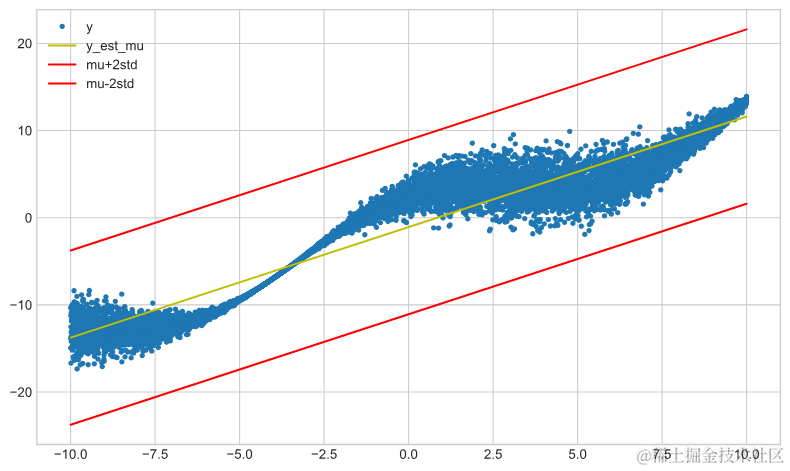
plot_modesults(mod_linreg......, tfp_model=False)
TensorFlow概率
我们可以通过最大化正态分布的似然性来拟合上述相同的模型,其中平均值是线性回归模型的估计值。
def negloglik(y, distr): ...... model_lin_reg_tfp = tf.keras.Sequential( ...... lambda t: tfp.distributions.Normal(loc=t, scale=5,) ), ] ) model_lin_reg_tfp.compile( ......) history = model_lin_reg_tf...... plot_model_results(model_lin_r......rue)
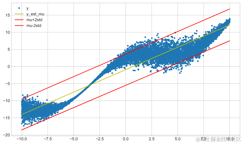
拟合带有标准差的线性回归
为了拟合线性回归模型的最佳标准差,我们需要进行一些操作。我们需要网络输出两个节点,一个用于表示平均值,另一个用于表示标准差。
model_lin_reg_std_tfp = tf.keras.Sequential(
    [
  ......
        ),
    ]
)

model_lin_reg_std_tfp.compile(
......)

history = model_lin_reg_std_tfp.fit(x_train, y_train, epochs=50, ......train, tfp_model=True)
model_lin_reg_std_nn_tfp = tf.keras.Sequential(
    [
 ......
            )
        ),
    ]
)

model_lin_reg_std_nn_tfp.compile(
   ......
plot_model_results(mode ......rain, tfp_model=True)
随时关注您喜欢的主题
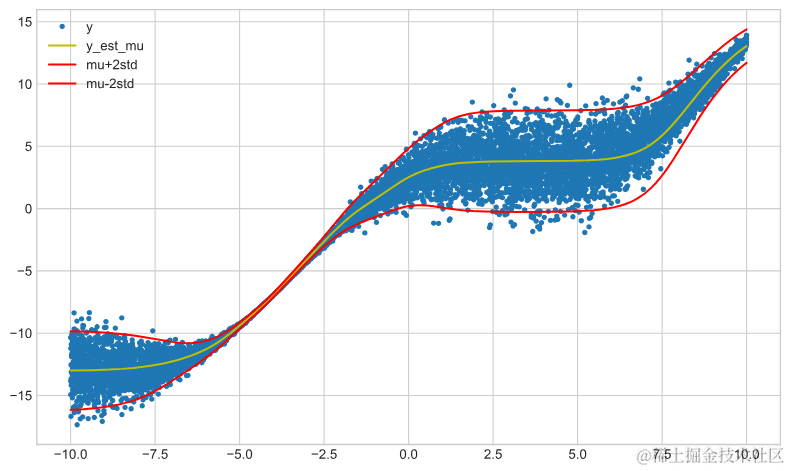
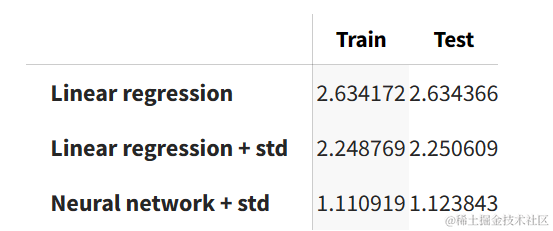
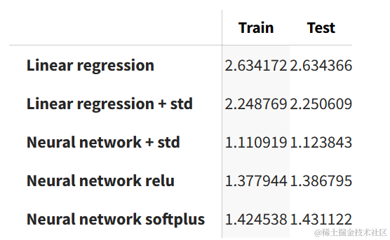
我们对训练集和测试集运行了各个模型。在任何模型中,两者之间的性能变化不大。我们可以看到,神经网络模型在训练集和测试集上的表现最好。
results = pd.DataFrame(index=["Train", "Test"])

models = {
  ......
        ).numpy(),
    ]
results.transpose()
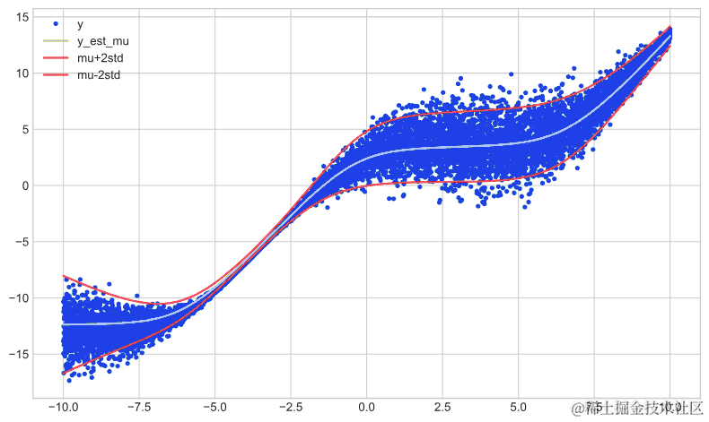
激活函数
下面使用relu或softplus激活函数创建相同的网络。首先是relu网络的结果:
model_relu = tf.keras.Sequential(
    [
  ......
                loc=t[:, 0:1], scale=tf.math.softplus(t[:, 1:2])
            )
        ),
    ]
)

m ......
plot_model_results(model_relu, x_train, y_train)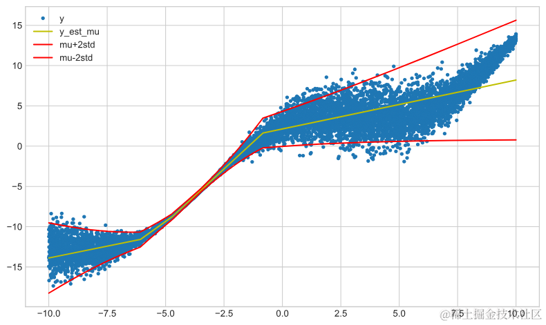
然后是softplus的结果:
model_softplus = tf.keras.Sequential(
    [
  ......
                loc=t[:, 0:1], scale=tf.math.softplus(t[:, 1:2])
            )
        ),
    ]
)

model_softplus.compile(
 ......
plot_model_results(model_softplus, x_train, y_train)
我们可以看到,基于sigmoid的神经网络具有最佳性能。
results = pd.DataFrame(index=["Train", "Test"])

models = {
 ......(x_test))
        ).numpy(),
    ]
results.transpose()
可下载资源
关于作者
Kaizong Ye是拓端研究室(TRL)的研究员。在此对他对本文所作的贡献表示诚挚感谢,他在上海财经大学完成了统计学专业的硕士学位,专注人工智能领域。擅长Python.Matlab仿真、视觉处理、神经网络、数据分析。
本文借鉴了作者最近为《R语言数据分析挖掘必知必会 》课堂做的准备。
非常感谢您阅读本文,如需帮助请联系我们!
 Python、R开发K-Means、CART、LR、SVM、BP神经网络五模型对比实现电信客户流失预测挽留|附AI智能体、代码和数据
 Python融合SVD矩阵分解与NCF神经协同过滤的电影评分预测与推荐系统|附AI智能体、代码和数据
 Python结合TF-IDF、逻辑回归、transformers、DistilBERT实现评论语义搜索|附AI智能体、代码和数据