对于线性关系,我们可以进行简单的线性回归。对于其他关系,我们可以尝试拟合一条曲线。
曲线拟合是构建一条曲线或数学函数的过程,它对一系列数据点具有最佳的拟合效果。
使用示例数据集
#我们将使Y成为因变量,X成为预测变量
#因变量通常在Y轴上
plot(x,y,pch=19)
可下载资源
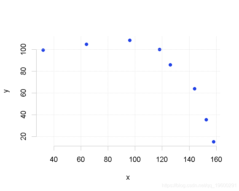
看起来我们可以拟合一条曲线。
#拟合一次多项式方程。

fit <- lm(y~x)

#二次

fit2 <- lm(y~poly(x,2)

#三次

......
#生成50个数字的范围,从30开始到160结束

xx <- seq(30,160, length=50)

lines(xx, predict(fit, xx)
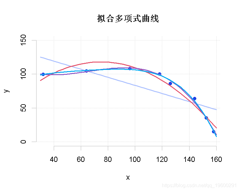
我们可以看到每条曲线的拟合程度。
我们可以使用summary()函数对拟合结果进行更详细的统计。
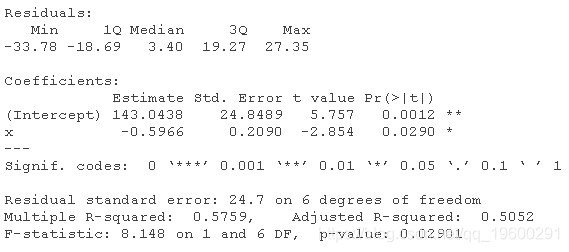
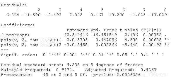
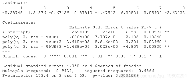
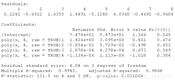
使用不同多项式R平方的总结。
1st: 0.5759
2nd: 0.9474
3rd: 0.9924
4th: 0.9943
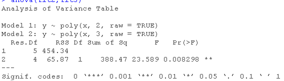
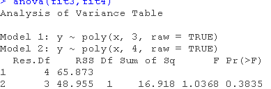
我们可以用 “方差分析 “来比较不同的模型。
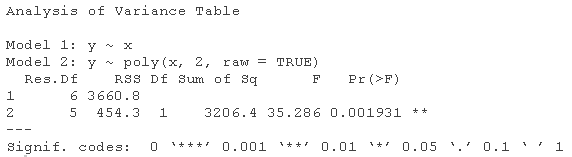
Pr(>F)值是拒绝无效假设的概率,即一个模型不比另一个模型更适合。我们有非常显著的P值,所以我们可以拒绝无效假设,即fit2比fit提供了更好的拟合。
随时关注您喜欢的主题
我们还可以创建一个反映多项式方程的函数。
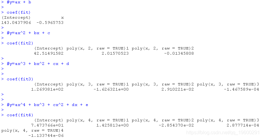
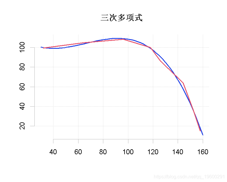
从三次多项式推算出来的数值与原始数值有很好的拟合,我们可以从R-squared值中得知。
结论
对于非线性曲线拟合,我们可以使用lm()和poly()函数,这也为多项式函数对数据集的拟合程度提供了有用的统计数据。我们还可以使用方差分析测试来评估不同模型之间的对比程度。从模型中可以定义一个反映多项式函数的函数,它可以用来推算因变量。
yy<-third(xx,fit)

plot(xx,yy)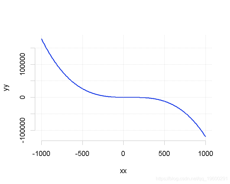
 2026年出海品牌平台迁移白皮书:寻找第二增长曲线|附100+数据、报告下载
 Python梯度提升树、XGBoost、LASSO回归、决策树、SVM、随机森林预测中国A股上市公司数据研发操纵融合CEO特质与公司特征及SHAP可解释性研究|附代码数据
 Python谷歌商店Google Play APP评分预测:LASSO、多元线性回归、岭回归模型对比研究