之前我们讨论了使用ROC曲线来描述分类器的优势,有人说它描述了“随机猜测类别的策略”。
让我们回到ROC曲线来说明,考虑一个非常简单的数据集,其中包含10个观测值(不可线性分离)。
在这里我们可以检查一下,确实是不可分离的。
plot(x1,x2,col=c("red","blue")[1+y],pch=19)roc曲线:接收者操作特征(receiver operating characteristic),roc曲线上每个点反映着对同一信号刺激的感受性。
针对一个二分类问题,将实例分成正类(postive)或者负类(negative)。但是实际中分类时,会出现四种情况(都是针对预测的类别来命名的).
(1)真正类(True Postive TP)(预测为正类,刚好预测的是正确的)
(2)假负类(False Negative FN)(预测为负类,只不过预测错了)
(3)假正类(False Postive FP)(预测为正类,只不过预测错了)
(4)真负类(True Negative TN)(预测为负类,刚好预测的是正确的)
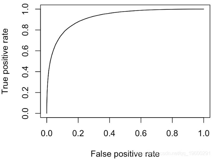
横轴:负正类率(false postive rate FPR)特异度,划分实例中所有负例占所有负例的比例;(1-Specificity)
纵轴:真正类率(true postive rate TPR)灵敏度,Sensitivity(正类覆盖率)(又是召回率recall)
由上表可得出横,纵轴的计算公式:
(1)真正类率(True Postive Rate)TPR: TP/(TP+FN),代表分类器预测的正类中实际正实例占所有正实例的比例。Sensitivity
(2)负正类率(False Postive Rate)FPR: FP/(FP+TN),代表分类器预测的正类中实际负实例占所有负实例的比例。1-Specificity
(3)真负类率(True Negative Rate)TNR: TN/(FP+TN),代表分类器预测的负类中实际负实例占所有负实例的比例,TNR=1-FPR。Specificity
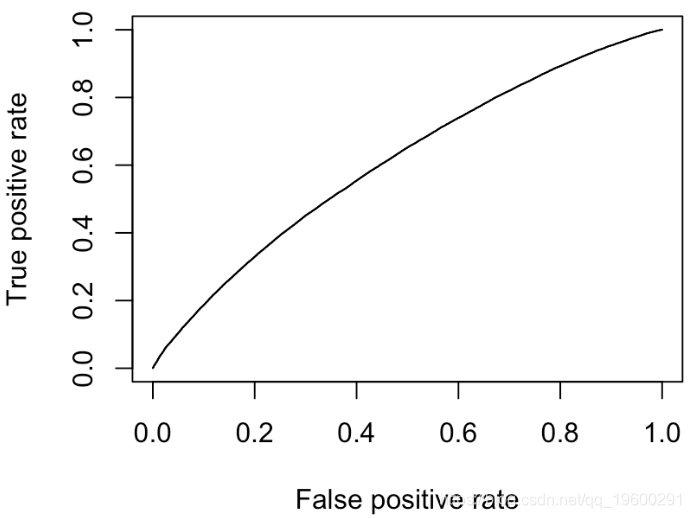
假设采用逻辑回归分类器,其给出针对每个实例为正类的概率,那么通过设定一个阈值如0.6,概率大于等于0.6的为正类,小于0.6的为负类。对应的就可以算出一组(FPR,TPR),在平面中得到对应坐标点。随着阈值的逐渐减小,越来越多的实例被划分为正类,但是这些正类中同样也掺杂着真正的负实例,即TPR和FPR会同时增大。阈值最大时,对应坐标点为(0,0),阈值最小时,对应坐标点(1,1)。
考虑逻辑回归
reg = glm(y~x1+x2,data=df,family=binomial(link = "logit"))
我们可以使用我们自己的roc函数
 roc=function(s,print=FALSE){
Ps=(S<=s)*1

FP=sum((Ps==1)*(Y==0)/sum(Y==0)

TP=sum((Ps==1)*(Y==1)/sum(Y==1)

if(print==TRUE){

print(table(Observed=Y,Predicted=Ps))


vect=c(FP,TP)

names(vect)=c("FPR","TPR")
或R包
performance(prediction(S,Y),"tpr","fpr")我们可以在这里同时绘制两个
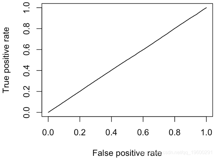
因此,我们的代码在这里可以正常工作。让我们考虑一下对角线。第一个是:每个人都有相同的概率(例如50%)
points(V[1,],V[2,])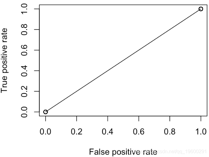
但是,我们这里只有两点:(0,0)和(1,1)。实际上,无论我们选择何种概率,都是这种情况
plot(performance(prediction(S,Y),"tpr","fpr"))
points(V[1,],V[2,])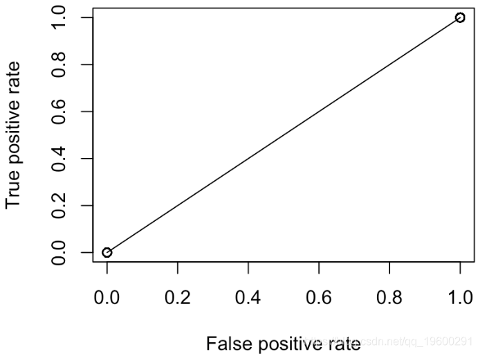

我们可以尝试另一种策略,例如“通过扔无偏硬币进行预测”。我们得到
segments(0,0,1,1,col="light blue")我们还可以尝试“随机分类器”,在其中我们随机选择分数
S=runif(10)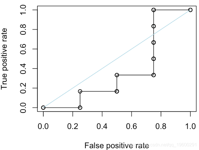
更进一步。我们考虑另一个函数来绘制ROC曲线
y=roc(x)
lines(x,y,type="s",col="red")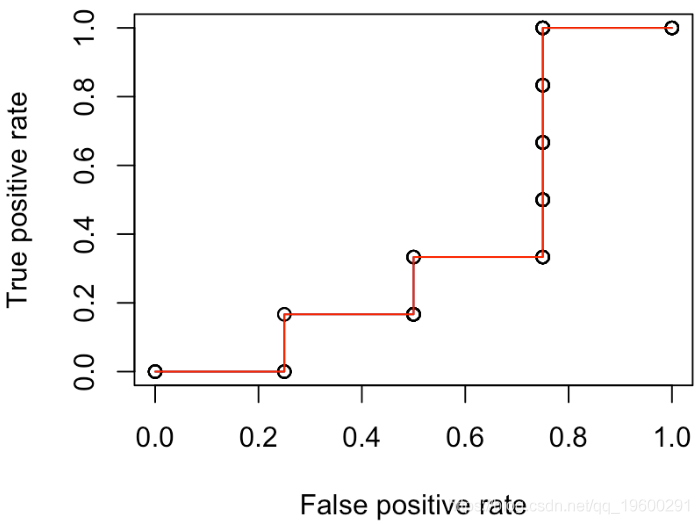
但是现在考虑随机选择的策略
for(i in 1:500){
S=runif(10)
V=Vectorize(roc.curve)(seq(0,1,length=251)
MY[i,]=roc_curve(x)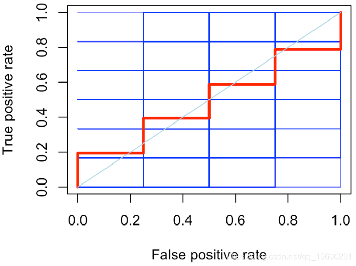
红线是所有随机分类器的平均值。它不是一条直线,我们观察到它在对角线周围的波动。
reg = glm(PRO~.,data=my,family=binomial(link = "logit"))


plot(performance(prediction(S,Y),"tpr","fpr"))


segments(0,0,1,1,col="light blue")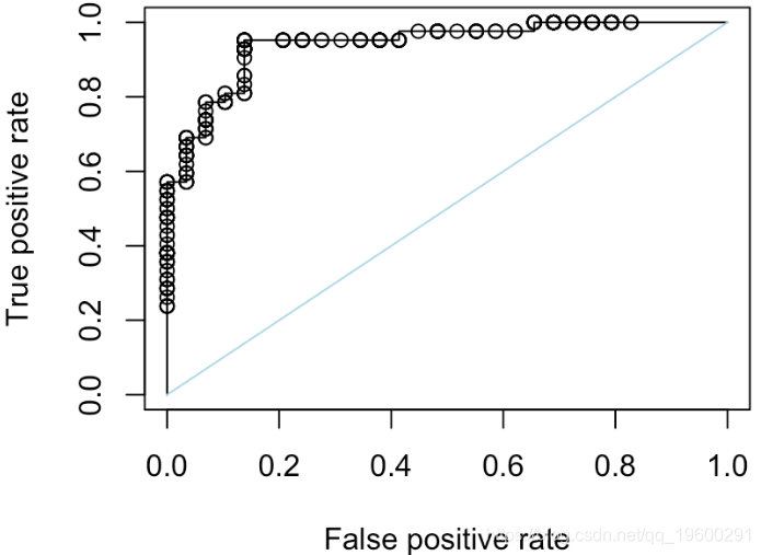
这是一个“随机分类器”,我们在单位区间上随机绘制分数
segments(0,0,1,1,col="light blue")如果我们重复500次,我们可以获得
for(i in 1:500){
S=runif(length(Y))
MY[i,]=roc(x)
}
lines(c(0,x),c(0,apply(MY,2,mean)),col="red",type="s",lwd=3)
segments(0,0,1,1,col="light blue")
因此,当我在单位区间上随机绘制分数时,就会得到对角线的结果。给定Y,我们可以绘制分数的两个经验累积分布函数
plot(f0,(0:(length(f0)-1))/(length(f0)-1))

lines(f1,(0:(length(f1)-1))/(length(f1)-1))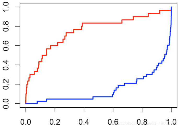
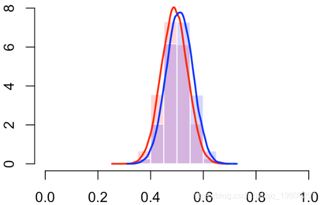
我们还可以使用直方图(或密度估计值)查看分数的分布
hist(S[Y==0],col=rgb(1,0,0,.2),
 probability=TRUE,breaks=(0:10)/10,border="white")
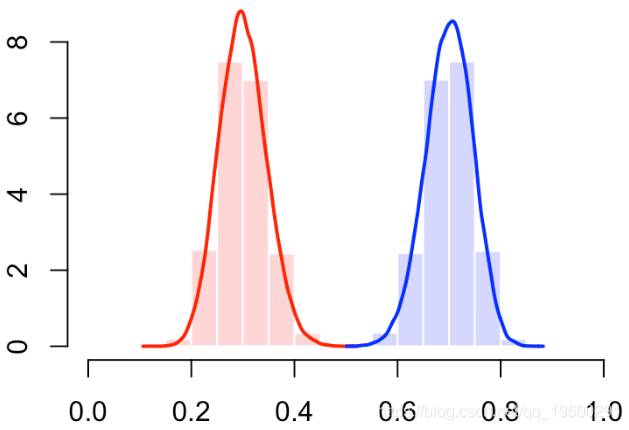
我们确实有一个“完美的分类器”(曲线靠近左上角)
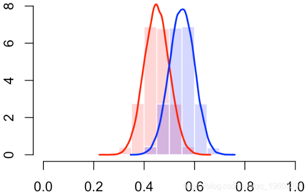
有错误。那应该是下面的情况
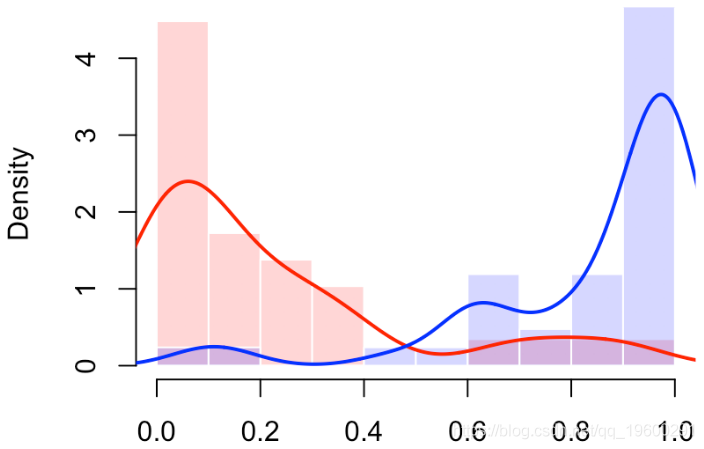
在10%的情况下,我们可能会分类错误
更多的错误分类
最终我们有对角线
 R语言与MATLAB定制开发SARIMAX双模型预测与PSO多目标优化消费券发放策略|附AI智能体、代码和数据
 Python随机森林、梯度提升树与逻辑回归融合多阶段特征工程实现信贷违约风险预测|附AI智能体、代码和数据
 Python结合TF-IDF、逻辑回归、transformers、DistilBERT实现评论语义搜索|附AI智能体、代码和数据
 居民健康调查数据|高血压慢性病影响因素识别:Python逻辑回归LR多层感知器MLP预测|附数据代码