在拟合 GLM(并检查残差)之后,可以使用 z 检验一一检验估计参数的显着性,即将估计值与其标准误差进行比较。
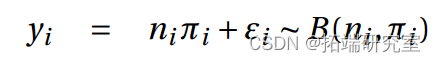
GLM 模型拟合和分析示例
示例 1. 小鼠数据的 GLM 建模(剂量和反应)
可下载资源
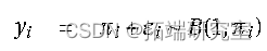
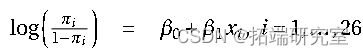
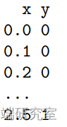
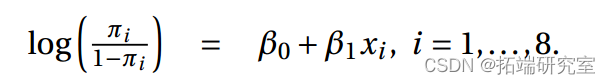
a) 我们输入数据并拟合逻辑回归模型。
此函数是 Bernoulli 在 GLM 的 response function,即 link function 的反函数。(强调反函数的时候可以使用 g−1(x)g−1(x) 标识;当然直接使用 g(x)g(x) 也没问题,Andrew 课上使用的是后者)
此函数在神经网络中也有用作 activate function 来引入非线性(当然现在更常用 rectified linear unit, RELU),其拥有一些特点:
bounded 有界的,取值 (0,1)(0,1),有概率意义
monotonic 单调递增函数
differentiable 可微,且求导简单
函数呈 S 曲线,中央区域敏感,两侧抑制(有俩个优点:首先是符合神经激活原理;其次是现实问题会有类似的非线性关系,当自变量很大或很小时对因变量影响很小,但是在某个阈值范围上时影响很大)
> summary(it1.lt)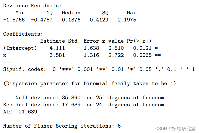
1-pchisq(17.6,24)
模型: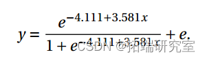
可以与完整模型进行比较。与偏差值 17.639 相关的 P 值 0.82(> 0.10)意味着没有显着证据拒绝拟合模型。
anova(fi.lgi)
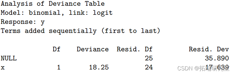
1-pchisq(35.8-17.69,25-24)
空模型不包含预测变量,在 25 个自由度 (df) 上的偏差为 35.89。当协变量 x 添加到空模型时,偏差的变化是 35.890-17.639=18.25。与自由度为 25-24=1 的卡方分布相比,其 P 值为 1.93 × 10 -5 非常显着。
因此模型不能通过删除 x 来简化。x 的系数的 t 检验也很重要(P 值 0.0065<0.01)。
截距呢?可以删掉吗?
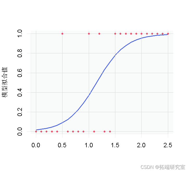
> plotx, itte(fi1log,typ"
> pot(,y
随时关注您喜欢的主题
图 1:逻辑回归的小鼠数据和拟合值。
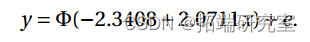
b)我们拟合一个带有概率链接的模型。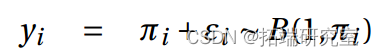

>summary()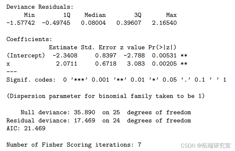
配套模型:
同样,这两个参数都很重要(P 值<0.01)
>anova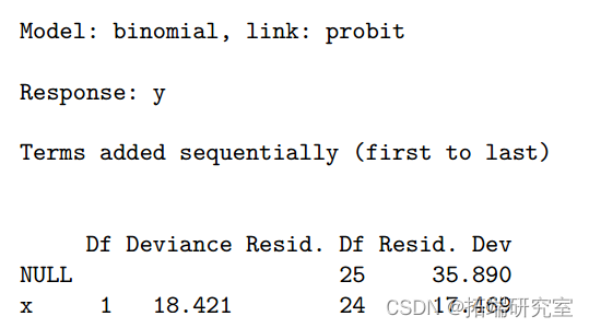
> 1 - pchisq(35.89-17.49 25-24)
>lines(x,fitte 添加 x 时偏差的变化是显着的(P 值 =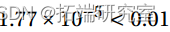 )。
)。
模型不能通过删除 x 来简化。
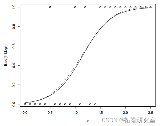
图 2:小鼠数据和拟合值(虚线:概率链接)。
使用 probit 链接的模型略好于使用 logit 链接的模型,因为偏差更小。在两个模型中,x 的系数都很显着(P 值<0.01),这意味着效果随着剂量的增加而增加。
示例 2. 临床试验数据(剂量和反应)的 GLM 建模。
a) 我们输入数据,然后拟合逻辑回归模型
>summary(it2.it)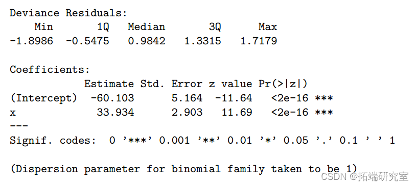
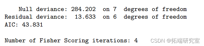
1-pchisq(13.63,6)
与偏差值 13.633 相关的 P 值为 0.034<0.05。5% 的水平拒绝拟合模型。
针对 x 绘制残差揭示了一种依赖模式。
>plot(x;reid(it2.it))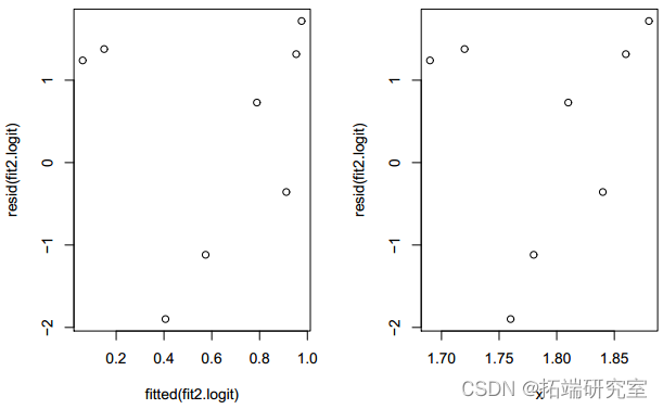
图 3:仅带有 x 的拟合模型的残差图。
plt(fitdft2lit;reid(fi2lot))所以我们将 x2 添加到模型中。
>;summary(ft2qlt)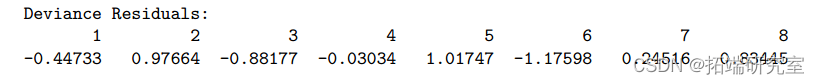
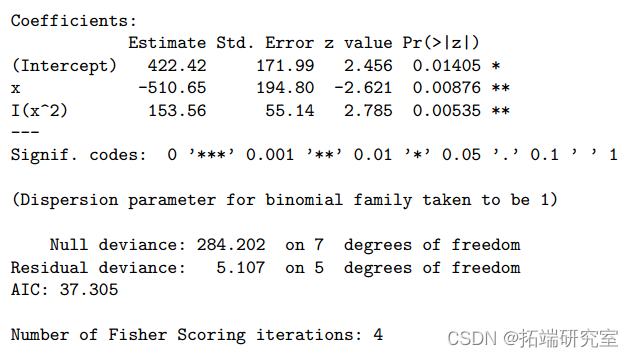
>;1-pchisq(5.1, 5)
偏差从 13.633 减少到 5.107,不显着(P 值=0.403>0.05)。
因此,我们不能通过偏差的证据来拒绝这个模型。
plot(fitted(fit2logit),resid(.logit))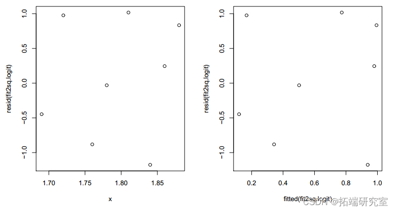
图 4:带有 x2 的拟合模型的残差图。
残差现在看起来是随机的。
拟合模型为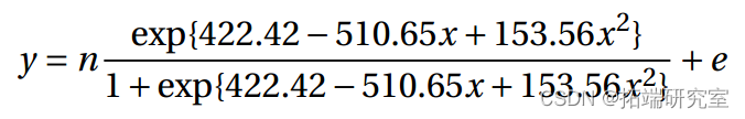
并且所有参数估计值都很显着(5%)。对数几率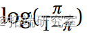 以二次方式依赖于 x。
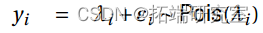
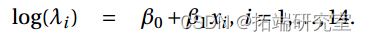
示例 3. 艾滋病数据,泊松
a) 我们输入数据并使用默认对数链接拟合泊松回归模型。
>smary(fit.lg)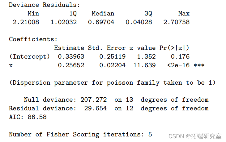
>1-pchisq
偏差 29.654 的 P 值为 0.005<0.01 ⇒ 模型被拒绝。
plot(fit3esuals)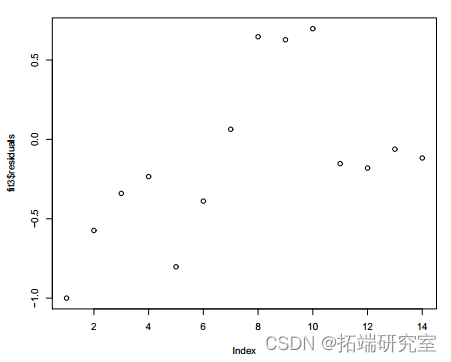
图 5:拟合模型 3
的残差图 b) 针对年份指数 x 的残差图显示了依赖模式。所以我们添加 .
.
>summary(fi3.lg)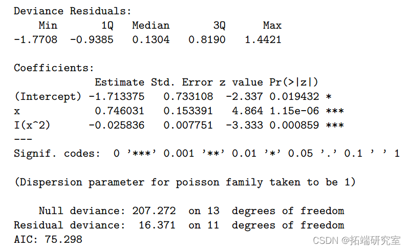
>1-pchisq

\[1\] 0.1279
16.371 的偏差(P 值为 0.1279>0.10)并不显着。拟合模型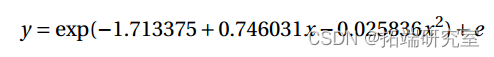
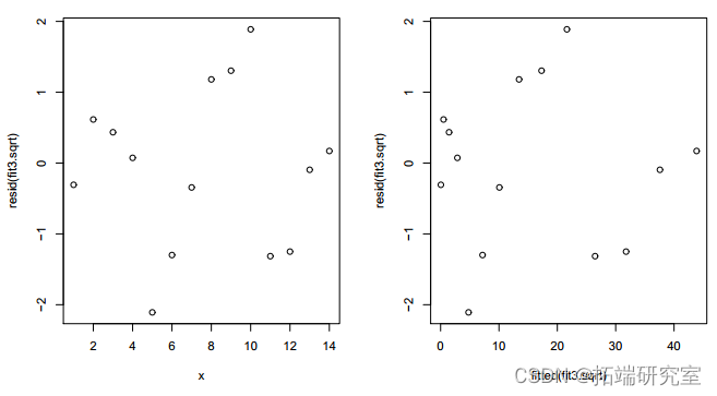
不能以偏差为由拒绝。但残差图只显示了比以前稍微随机的模式。

图 6:拟合模型 3 与 x2 的残差图
该模型可以通过使用非规范链接进行改进。
> summary(ft3st)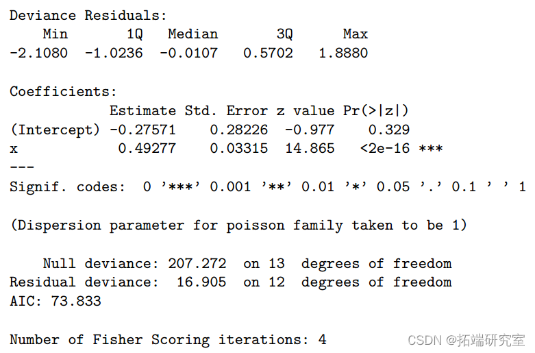
> 1 - pchisq(16.9, 12)
[1] 0.153
拟合模型的残差 y = (-0.27571 +0.49277x)2 + e 显示出更加随机的模式。12 df 上的偏差 16.905 略高于之前模型的 16.371(df=11),但仍然不显着(P 值=0.1532>0.10)。AIC 较小,为 73.833<75.298。因此,具有平方根链接的模型是首选。
可以删除常数项(“截距”)吗?
还可以使用哪些其他链接功能?
自测题:
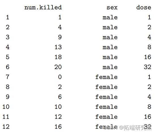
Twenty tobacco budworm moths of each sex were exposed to different doses of the insecticide trans-cypermethrin. The numbers of budworm moths killed during a 3-day exposure were as follows for each sex (male, female) and dose level in mg’s.
Type the data into R as follows. Press Enter at the end of each line including blank lines.
num.killed <- scan()
1 4 9 13 18 20 0 2 6 10 12 16
sex <- scan()
0 0 0 0 0 0 1 1 1 1 1 1
dose <- scan()
1 2 4 8 16 32 1 2 4 8 16 32
Fit two models by doing the following.
ldose <- log(dose)/log(2) #convert to base-2 log dose
ldose #have a look
y <- cbind(num.killed, 20-num.killed) #add number survived
fit1 <- glm(y ~ ldose * sex, family=binomial(link=probit))
fit2 <- glm(y ~ sex + ldose, family=binomial(link=probit))
You may also run the following lines and refer to the chi-square distribution table
anova(fit1,test="Chisq")

summary(fit2)
1. What model is fitted in fit1? Write it formally and define all the terms.
2. How is the model in fit2 differ from that in fit1?
3. Does the model in fit1 fit the data adequately? Use deviance to answer this question.
4. Can the model in fit1 be simplified to the model in fit2? Use change in deviance to answer
this question.
5. Can sex be removed from the model in fit2? Use change in deviance to answer this ques
tion.
6. What are the maximum likelihood estimates of the parameters of the additive model? What
are their standard errors? Test the significance of each parameter using its estimate and
standard error.
7. How does the probability of a kill change with log dose and sex of the budworm moth accord
ing to the additive model?
(a) Derive the survival function S(t) of a lifetime T » E xp(‚). Find ¡logS(t) and comment on it.
(b) Calculate the Kaplan-Meier estimate for each group in the following.
Treatment Group:
6,6,6,6,7,9,10,10,11,13,16,17,19,20,22,23,25,32,32,34*,35
Control Group (no treatment):
1,1,2,2,3,4,5,5,8,8,8,8,11,11,12,15,17,22,23
Note that * indicates right censored data.
(c) Use the log rank test to compare the two groups of lifetimes.
可下载资源
关于作者
Kaizong Ye是拓端研究室(TRL)的研究员。在此对他对本文所作的贡献表示诚挚感谢,他在上海财经大学完成了统计学专业的硕士学位,专注人工智能领域。擅长Python.Matlab仿真、视觉处理、神经网络、数据分析。
本文借鉴了作者最近为《R语言数据分析挖掘必知必会 》课堂做的准备。
非常感谢您阅读本文,如需帮助请联系我们!
 2026汽车出海行业深度报告:新能源出口、全球区域布局、电动两轮车|附200+报告数据合集下载
 Python结合TF-IDF、逻辑回归、transformers、DistilBERT实现评论语义搜索|附AI智能体、代码和数据
 2026年数字化数智化转型趋势报告:价值、AI落地与风险平衡 | 附200+报告、数据合集下载
 Python融合RNN、GRU、LSTM多变量空气质量多步预测|附AI智能体、代码和数据