
我尝试使用Latent Dirichlet分配LDA来提取一些主题。 本教程以自然语言处理流程为特色,从原始数据开始,准备,建模,可视化论文。
我们将涉及以下几点:1.使用LDA进行主题建模。2.使用pyLDAvis可视化主题模型。3.使用t-SNE可视化LDA结果。
from scipy import sparse as sp
Populating the interactive namespace from numpy and matplotlib
-
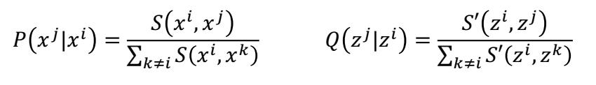
t-SNE(t-distributed stochastic neighbor embedding)是用于降维的一种机器学习算法,是由 Laurens van der Maaten 和 Geoffrey Hinton在08年提出来。此外,t-SNE 是一种非线性降维算法,非常适用于高维数据降维到2维或者3维,进行可视化。相对于PCA来说,t-SNE可以说是一种更高级有效的方法,在第二部分我们会展示t-SNE和PCA在手写数字体上的效果对比。
-
原理简述:t-SNE是一种降维算法,目的就是把X(原始高维数据)转换成Z(指定低维度的数据)。t-SNE首先将距离转换为条件概率来表达点与点之间的相似度,距离通过欧式距离算得,S(
,
)表示求
之间的欧式距离。计算原始高维数据X与转换后的低维数据Z的公式如下所示。
计算完X数据之间的的概率P( )和Z数据之间的概率Q(
|
)之后,接下来就是我们 的目的就是P和Q连个分布尽可能的接近,也就是要是如下公式的KL散度尽可能小。
docs = array(p_df['PaperText'])
预处理和矢量化文档
from nltk.stem.wordnet import WordNetLemmatizer
from nltk.tokenize import RegexpTokenizer

def docs_preprocessor(docs):
    tokenizer = RegexpTokenizer(r'\w+')
    for idx in range(len(docs)):
        docs[idx] = docs[idx].lower()  # Convert to lowercase.
        docs[idx] = tokenizer.tokenize(docs[idx])  # Split into words.

    # 删除数字,但不要删除包含数字的单词。

    docs = [[token for token in doc if not token.isdigit()] for doc in docs]

    # 删除仅一个字符的单词。

    docs = [[token for token in doc if len(token) > 3] for doc in docs]

    # 使文档中的所有单词规则化

    lemmatizer = WordNetLemmatizer()
    docs = [[lemmatizer.lemmatize(token) for token in doc] for doc in docs]

return docsdocs = docs_preprocessor(docs)
计算双字母组/三元组:

主题非常相似,可以区分它们是短语而不是单个单词。
In [5]:
from gensim.models import Phrases
# 向文档中添加双字母组和三字母组(仅出现10次或以上的文档)。
bigram = Phrases(docs, min_count=10)
trigram = Phrases(bigram[docs])

for idx in range(len(docs)):
    for token in bigram[docs[idx]]:
        if '_' in token:
            # Token is a bigram, add to document.
            docs[idx].append(token)
    for token in trigram[docs[idx]]:
        if '_' in token:
            # token是一个二元组,添加到文档中。
            docs[idx].append(token)
Using TensorFlow backend.
/opt/conda/lib/python3.6/site-packages/gensim/models/phrases.py:316: UserWarning: For a faster implementation, use the gensim.models.phrases.Phraser class
warnings.warn("For a faster implementation, use the gensim.models.phrases.Phraser class")删除
In [6]:
from gensim.corpora import Dictionary

# 创建文档的字典表示

dictionary = Dictionary(docs)
print('Number of unique words in initital documents:', len(dictionary))

# 过滤掉少于10个文档或占文档20%以上的单词。

dictionary.filter_extremes(no_below=10, no_above=0.2)
print('Number of unique words after removing rare and common words:', len(dictionary))
Number of unique words in initital documents: 39534
Number of unique words after removing rare and common words: 6001清理常见和罕见的单词,我们最终只有大约6%的词。

矢量化数据:
第一步是获得每个文档的单词表示。
In [7]:
corpus = [dictionary.doc2bow(doc) for doc in docs]
In [8]:
print('Number of unique tokens: %d' % len(dictionary))
print('Number of documents: %d' % len(corpus))
Number of unique tokens: 6001
Number of documents: 403通过词袋语料库,我们可以继续从文档中学习我们的主题模型。
训练LDA模型
In [9]:
from gensim.models import LdaModel
In [10]:
%time model = LdaModel(corpus=corpus, id2word=id2word, chunksize=chunksize, \
                       alpha='auto', eta='auto', \
                       iterations=iterations, num_topics=num_topics, \
                       passes=passes, eval_every=eval_every)
CPU times: user 3min 58s, sys: 348 ms, total: 3min 58s
Wall time: 3min 59s随时关注您喜欢的主题
如何选择主题数量?
LDA是一种无监督的技术,这意味着我们在运行模型之前不知道在我们的语料库中有多少主题存在。 主题连贯性是用于确定主题数量的主要技术之一。
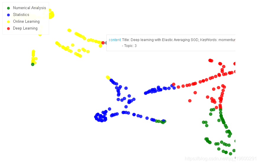
但是,我使用了LDA可视化工具pyLDAvis,尝试了几个主题并比较了结果。 四个似乎是最能分离主题的最佳主题数量。
In [11]:
import pyLDAvis.gensim
pyLDAvis.enable_notebook()

import warnings
warnings.filterwarnings("ignore", category=DeprecationWarning)
In [12]:
pyLDAvis.gensim.prepare(model, corpus, dictionary)
Out[12]:
我们在这看到什么?
左侧面板,标记为Intertopic Distance Map,圆圈表示不同的主题以及它们之间的距离。类似的主题看起来更近,而不同的主题更远。图中主题圆的相对大小对应于语料库中主题的相对频率。
如何评估我们的模型?
将每个文档分成两部分,看看分配给它们的主题是否类似。 =>越相似越好
将随机选择的文档相互比较。 =>越不相似越好
In [13]:
from sklearn.metrics.pairwise import cosine_similarity

p_df['tokenz'] = docs

docs1 = p_df['tokenz'].apply(lambda l: l[:int0(len(l)/2)])
docs2 = p_df['tokenz'].apply(lambda l: l[int0(len(l)/2):])
转换数据
In [14]:
corpus1 = [dictionary.doc2bow(doc) for doc in docs1]
corpus2 = [dictionary.doc2bow(doc) for doc in docs2]

# 使用语料库LDA模型转换


lda_corpus1 = model[corpus1]
lda_corpus2 = model[corpus2]
In [15]:
from collections import OrderedDict
def get_doc_topic_dist(model, corpus, kwords=False):

    '''
LDA转换,对于每个文档,仅返回权重非零的主题
此函数对主题空间中的文档进行矩阵转换
    '''
    top_dist =[]
    keys = []

    for d in corpus:
        tmp = {i:0 for i in range(num_topics)}
        tmp.update(dict(model[d]))
        vals = list(OrderedDict(tmp).values())
        top_dist += [array(vals)]
        if kwords:
            keys += [array(vals).argmax()]

    return array(top_dist), keys
Intra similarity: cosine similarity for corresponding parts of a doc(higher is better):
0.906086532099
Inter similarity: cosine similarity between random parts (lower is better):
0.846485334252
让我们看一下每个主题中出现的单词。
In [17]:
def explore_topic(lda_model, topic_number, topn, output=True):
    """


输出topn词的列表
    """
    terms = []
    for term, frequency in lda_model.show_topic(topic_number, topn=topn):
        terms += [term]
        if output:
            print(u'{:20} {:.3f}'.format(term, round(frequency, 3)))

    return terms
In [18]:
term frequency
Topic 0 |---------------------
data_set 0.006
embedding 0.004
query 0.004
document 0.003
tensor 0.003
multi_label 0.003
graphical_model 0.003
singular_value 0.003
topic_model 0.003
margin 0.003
Topic 1 |---------------------
policy 0.007
regret 0.007
bandit 0.006
reward 0.006
active_learning 0.005
agent 0.005
vertex 0.005
item 0.005
reward_function 0.005
submodular 0.004
Topic 2 |---------------------
convolutional 0.005
generative_model 0.005
variational_inference 0.005
recurrent 0.004
gaussian_process 0.004
fully_connected 0.004
recurrent_neural 0.004
hidden_unit 0.004
deep_learning 0.004
hidden_layer 0.004
Topic 3 |---------------------
convergence_rate 0.007
step_size 0.006
matrix_completion 0.006
rank_matrix 0.005
gradient_descent 0.005
regret 0.004
sample_complexity 0.004
strongly_convex 0.004
line_search 0.003
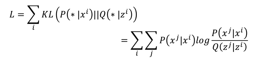
sample_size 0.003从上面可以检查每个主题并为其分配一个可解释的标签。 在这里我将它们标记如下:
In [19]:
top_labels = {0: 'Statistics', 1:'Numerical Analysis', 2:'Online Learning', 3:'Deep Learning'}
In [20]:
  '''
    # 1.删除非字母


    paper_text = re.sub("[^a-zA-Z]"," ", paper)
    # 2.将单词转换为小写并拆分


    words = paper_text.lower().split()
    # 3. 删除停用词


    words = [w for w in words if not w in stops]
    # 4. 删除短词


    words = [t for t in words if len(t) > 2]
    # 5. 形容词


    words = [nltk.stem.WordNetLemmatizer().lemmatize(t) for t in words]
In [21]:
from sklearn.feature_extraction.text import TfidfVectorizer

tvectorizer = TfidfVectorizer(input='content', analyzer = 'word', lowercase=True, stop_words='english',\
                                  tokenizer=paper_to_wordlist, ngram_range=(1, 3), min_df=40, max_df=0.20,\
                                  norm='l2', use_idf=True, smooth_idf=True, sublinear_tf=True)

dtm = tvectorizer.fit_transform(p_df['PaperText']).toarray()
In [22]:
top_dist =[]
for d in corpus:
    tmp = {i:0 for i in range(num_topics)}
    tmp.update(dict(model[d]))
    vals = list(OrderedDict(tmp).values())
    top_dist += [array(vals)]
In [23]:
top_dist, lda_keys= get_doc_topic_dist(model, corpus, True)
features = tvectorizer.get_feature_names()
In [24]:
top_ws = []
for n in range(len(dtm)):
    inds = int0(argsort(dtm[n])[::-1][:4])
    tmp = [features[i] for i in inds]

    top_ws += [' '.join(tmp)]


cluster_colors = {0: 'blue', 1: 'green', 2: 'yellow', 3: 'red', 4: 'skyblue', 5:'salmon', 6:'orange', 7:'maroon', 8:'crimson', 9:'black', 10:'gray'}

p_df['colors'] = p_df['clusters'].apply(lambda l: cluster_colors[l])
In [25]:
from sklearn.manifold import TSNE
tsne = TSNE(n_components=2)
X_tsne = tsne.fit_transform(top_dist)
In [26]:
p_df['X_tsne'] =X_tsne[:, 0]
p_df['Y_tsne'] =X_tsne[:, 1]
In [27]:
from bokeh.plotting import figure, show, output_notebook, save#, 输出文件
from bokeh.models import HoverTool, value, LabelSet, Legend, ColumnDataSource
output_notebook()
BokehJS 0.12.5成功加载。
In [28]:
source = ColumnDataSource(dict(
    x=p_df['X_tsne'],
    y=p_df['Y_tsne'],
    color=p_df['colors'],
    label=p_df['clusters'].apply(lambda l: top_labels[l]),
#     msize= p_df['marker_size'],
    topic_key= p_df['clusters'],
    title= p_df[u'Title'],
    content = p_df['Text_Rep']
))
In [29]:
title = 'T-SNE visualization of topics'


plot_lda.scatter(x='x', y='y', legend='label', source=source,
                 color='color', alpha=0.8, size=10)#'msize', )

show(plot_lda)
可下载资源
关于作者
Kaizong Ye是拓端研究室(TRL)的研究员。在此对他对本文所作的贡献表示诚挚感谢,他在上海财经大学完成了统计学专业的硕士学位,专注人工智能领域。擅长Python.Matlab仿真、视觉处理、神经网络、数据分析。
本文借鉴了作者最近为《R语言数据分析挖掘必知必会 》课堂做的准备。
非常感谢您阅读本文,如需帮助请联系我们!
 高维变量选择专题|R、Python用HOLP、Lasso、SCAD、PCR、ElasticNet实例合集分析企业财务、糖尿病、基因数据
 PCA主成分分析原理与水果成熟状态数据分析实例:Python中PCA-LDA与卷积神经网络CNN
 R语言拟合线性混合效应模型、固定效应、随机效应参数估计可视化生物生长、发育、繁殖影响因素
 R语言逻辑回归、GAM、LDA、KNN、PCA主成分分析分类预测房价及交叉验证