假设条件

广义线性模型的假设少于大多数常见的参数检验。观测值仍然需要独立，并且需要指定正确的链接函数。因此，例如应该了解何时使用泊松回归以及何时使用逻辑回归。但是，不需要数据或残差的正态分布。

并非所有比例或计数都适用于逻辑回归分析

一个不采用逻辑回归的例子中，饮食研究中人们减肥的体重无法用初始体重的比例来解释作为“成功”和“失败”的计数。在这里，只要满足模型假设，就可以使用常用的参数方法。

过度分散

使用广义线性模型时要注意的一个潜在问题是过度分散。当模型的残余偏差相对于残余自由度较高时，就会发生这种情况。这基本上表明该模型不能很好地拟合数据。 

但是据我了解，从技术上讲，过度分散对于简单的逻辑回归而言不是问题，即具有二项式因果关系和单个连续自变量的问题。

伪R平方

对于广义线性模型（glm），R不产生r平方值。pscl  包中的  pR2  可以产生伪R平方值。

测试p值

检验逻辑对数或泊松回归的p值使用卡方检验。方差分析  来测试每一个系数的显着性。似然比检验也可以用来检验整体模型的重要性。

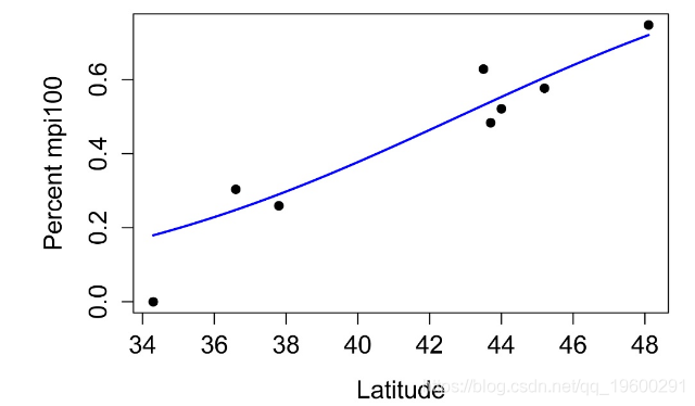
Logistic回归示例

Data = read.table(textConnection(Input),header=TRUE)

Data$Total = Data$mpi90 + Data$mpi100

Data$Percent = Data$mpi100 / + Data$Total

模型拟合

Trials = cbind(Data$mpi100, Data$mpi90)         # Sucesses, Failures

model = glm(Trials ~ Latitude, 
            data = Data, 
            family = binomial(link="logit"))

系数和指数系数

Coefficients:

            Estimate Std. Error z value Pr(>|z|)   

(Intercept) -7.64686    0.92487  -8.268   <2e-16 ***

Latitude     0.17864    0.02104   8.490   <2e-16 ***

 

 


                 2.5 %     97.5 %

(Intercept) -9.5003746 -5.8702453

Latitude     0.1382141  0.2208032

 

 
 # exponentiated coefficients

 

(Intercept)     Latitude

0.0004775391 1.1955899446

 

 
 # 95% CI for exponentiated coefficients

 

                   2.5 %      97.5 %

(Intercept) 7.482379e-05 0.002822181

Latitude    1.148221e+00 1.247077992

方差分析 

Analysis of Deviance Table (Type II tests)

 

Response: Trials

          Df  Chisq Pr(>Chisq)   

Latitude   1 72.076  < 2.2e-16 ***

伪R平方

$Models

                                                                

Model: "glm, Trials ~ Latitude, binomial(link = \"logit\"), Data"

Null:  "glm, Trials ~ 1, binomial(link = \"logit\"), Data"      

 

$Pseudo.R.squared.for.model.vs.null

                             Pseudo.R.squared

McFadden                             0.425248

Cox and Snell (ML)                   0.999970

Nagelkerke (Cragg and Uhler)         0.999970

模型的整体p值

 

Analysis of Deviance Table

 

Model 1: Trials ~ Latitude

Model 2: Trials ~ 1

  Resid. Df Resid. Dev Df Deviance  Pr(>Chi)   

1         6     70.333                         

2         7    153.633 -1  -83.301 < 2.2e-16 ***

 


Likelihood ratio test

 

Model 1: Trials ~ Latitude

Model 2: Trials ~ 1

  #Df  LogLik Df  Chisq Pr(>Chisq)   

1   2 -56.293                        

2   1 -97.944 -1 83.301  < 2.2e-16 ***

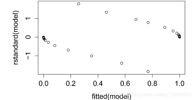
标准化残差图

 ​

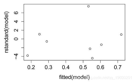
标准化残差与预测值的关系图。残差应无偏且均等。 

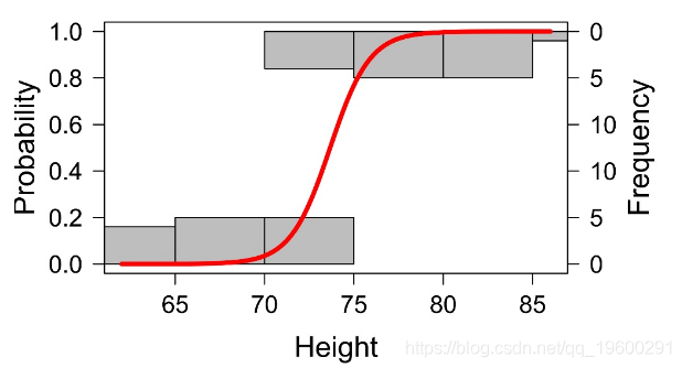
绘制模型

 ​

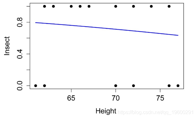
Logistic回归示例

Data = read.table(textConnection(Input),header=TRUE)

 

模型拟合

model 

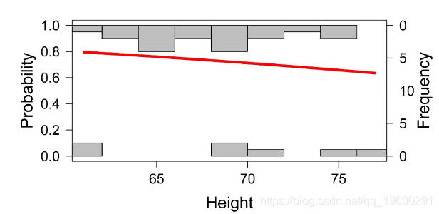
系数和指数系数

Coefficients:

            Estimate Std. Error z value Pr(>|z|)

(Intercept)  4.41379    6.66190   0.663    0.508

Height      -0.05016    0.09577  -0.524    0.600

 

 


 

                 2.5 %     97.5 %

(Intercept) -8.4723648 18.4667731

Height      -0.2498133  0.1374819

 

  # exponentiated coefficients

 

(Intercept)      Height

 82.5821122   0.9510757

 

 
 # 95% CI for exponentiated coefficients

 

                   2.5 %       97.5 %

(Intercept) 0.0002091697 1.047171e+08

Height      0.7789461738 1.147381e+0

 

方差分析

Analysis of Deviance Table (Type II tests)

 

Response: Insect

          Df  Chisq Pr(>Chisq)

Height     1 0.2743     0.6004

Residuals 23

伪R平方

$Pseudo.R.squared.for.model.vs.null

                             Pseudo.R.squared

McFadden                           0.00936978

Cox and Snell (ML)                 0.01105020

Nagelkerke (Cragg and Uhler)       0.01591030

模型的整体p值

Analysis of Deviance Table

 

Model 1: Insect ~ Height

Model 2: Insect ~ 1

  Resid. Df Resid. Dev Df Deviance Pr(>Chi)

1        23     29.370                    

2        24     29.648 -1 -0.27779   0.5982

 

 
 

Likelihood ratio test

 

Model 1: Insect ~ Height

Model 2: Insect ~ 1

  #Df  LogLik Df  Chisq Pr(>Chisq)

1   2 -14.685                     

2   1 -14.824 -1 0.2778     0.5982

标准化残差图

 ​

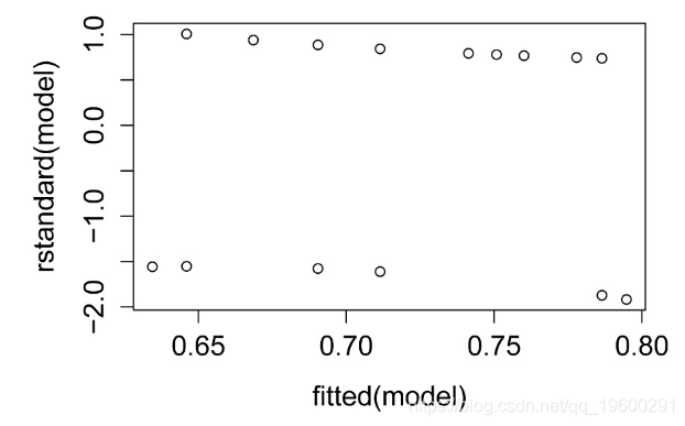
绘制模型

 

   Height Insect Insect.num

1      62 beetle          0

2      66  other          1

3      61 beetle          0

23     72  other          1

24     70 beetle          0

25     74  other          1

 

 ​

 

   Height Insect Insect.num Insect.log

1      62 beetle          0      FALSE

2      66  other          1       TRUE

3      61 beetle          0      FALSE

23     72  other          1       TRUE

24     70 beetle          0      FALSE

25     74  other          1       TRUE

 ​

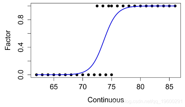
Logistic回归示例

Data = read.table(textConnection(Input),header=TRUE)


model

Coefficients:

            Estimate Std. Error z value Pr(>|z|) 

(Intercept) -66.4981    32.3787  -2.054   0.0400 *

Continuous    0.9027     0.4389   2.056   0.0397 *

 

 
 

Analysis of Deviance Table (Type II tests)

 

Response: Factor

           Df Chisq Pr(>Chisq) 

Continuous  1 4.229    0.03974 *

Residuals  27                  

 

 

                             Pseudo.R.squared

McFadden                             0.697579

Cox and Snell (ML)                   0.619482

Nagelkerke (Cragg and Uhler)         0.826303

 

 
 

  Resid. Df Resid. Dev Df Deviance Pr(>Chi)   

1        27     12.148                        

2        28     40.168 -1   -28.02  1.2e-07 ***

 

 

​ 

将因子转换为数字变量，级别为0和1 

   Continuous Factor Factor.num

1          62      A          0

2          63      A          0

3          64      A          0

27         84      B          1

28         85      B          1

29         86      B          1

 

 ​

将Factor转换为逻辑变量，级别为TRUE和FALSE 

 

   Continuous Factor Factor.num Factor.log

1          62      A          0      FALSE

2          63      A          0      FALSE

3          64      A          0      FALSE

27         84      B          1       TRUE

28         85      B          1       TRUE

29         86      B          1       TRUE

 

​