R语言用Backfitting MCMC抽样算法进行贝叶斯推理案例

BART是贝叶斯非参数模型，可以使用Backfitting MCMC进行拟合 。 

 我不使用任何软件包…… MCMC是从头开始实现的。

考虑协变量数据​和成果​为​主题，​。在这个 示例中，数据看起来像这样：

​

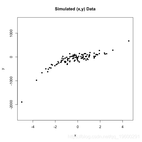
我们可能会考虑以下概率模型

 ​

​

基本上我们使用三次多项式对条件均值进行建模。请注意，这是更一般的 模型的特例

​

在这种情况下​和​。该模型​在参数矢量的每个元素上具有平坦的先验和在方差参数上具有形状和速率​的反伽马先验。​​​

每个条件后验​都是高斯（因为共轭）。我们可以使用共轭Gibbs或Metropolis从中进行采样。我们也可以将整个参数矢量​作为一个块进行采样，但是在这篇文章中我们将坚持反向拟合 – 这本身就是一个Gibbs采样器。我们仍然从其他条件的每个​条件的条件后验中进行抽样​。然而，我们利用关键的洞察力，每个条件后验​取决于其他beta ​，仅由残差表示

​

直观地，​是在减去​其他项（非​）所解释的部分之后的左手平均值的部分。它也是正常分布的，

​

在正常之前​，后验可以通过共轭来计算

​

Backfitting MCMC如下进行。首先，初始化所有测试版除外​。这完全是任意的 – 您可以从任何参数开始。然后，在每个Gibbs迭代中，

1. 计算​与值​在当前迭代。来自后验的样本  ​以电流抽取为条件​。
2. 计算​与值​在当前迭代。注意，​使用步骤1中的值。来自后部的样本  ​。
3. 对所有beta参数继续此过程。
4. ​绘制完所有参数后，进行采样​。这个后验是另一个反伽马。

术语反向拟合似乎是合适的，因为在每次迭代中，我们都“退出” ​我们想要使用其他测试版进行采样的分布。

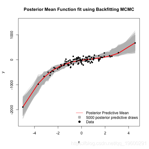
为了获得拟合的回归线，我们需要从后验预测分布中进行采样。我们在每个Gibbs迭代中的步骤4之后通过绘制​值来执行此操作

​

上标​表示使用来自​Gibbs迭代的值的参数。