自回归条件异方差(ARCH)模型涉及具有时变异方差的时间序列,其中方差是以特定时间点的现有信息为条件的。
ARCH模型假设时间序列模型中误差项的条件均值是常数(零),与我们迄今为止讨论的非平稳序列不同),但其条件方差不是。
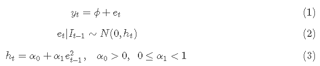
ARCH模型
这样一个模型可以用公式1、2和3来描述。
可下载资源
方程4和5给出了测试模型和假设,以测试时间序列中的ARCH效应,其中残差e^t来自于将变量yt回归一个常数,如1,或回归一个常数加上其他回归因子;方程4中的测试可能包括几个滞后项,在这种情况下,无效假设(方程5)是所有这些项都不显著。
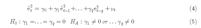
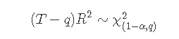
无效假设是不存在ARCH效应。检验统计量为

下面的例子使用了数据集,它包含了500个股票收益率的生成观测值。图显示了数据的时间序列图和柱状图。
plot.ts(r)
hist(r)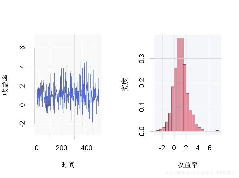
图: 变量 的水平和柱状图
让我们首先对数据集中的变量r一步一步地进行公式4和5中描述的ARCH检验。
summary(yd)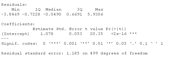
ehsq <- ts(resid(mean)^2)
summary(ARCH)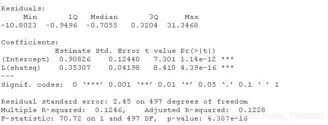
Rsq <- glance(ARCH)\[\[1\]\]
LM <- (T-q)*Rsq
Chicr <- qchisq(1-alpha, q)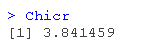
结果是LM统计量,等于62.16,与α=0.05和q=1自由度的临界卡方值进行比较;这个值是χ2(0.95,1)=3.84;这表明拒绝了无效假设,结论是该序列具有ARCH效应。
如果我们不使用一步步的程序,而是使用R的ARCH检验功能之一,也可以得出同样的结论。
ArchTest

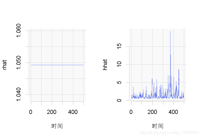
函数garch(),当使用order=参数等于c(0,1)时,成为一个ARCH模型。这个函数可以用来估计和绘制方程3中定义的方差ht,如以下代码和图所示。
garch(r,c(0,1))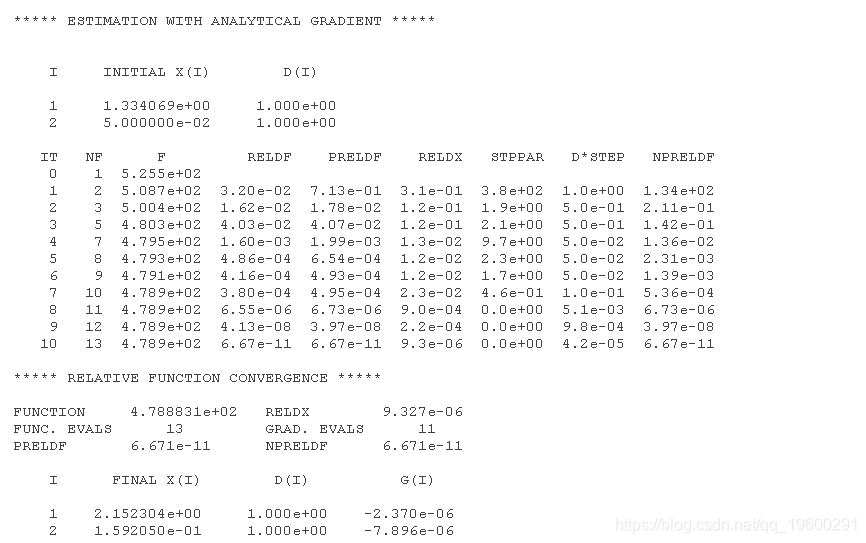
随时关注您喜欢的主题
summary(arch)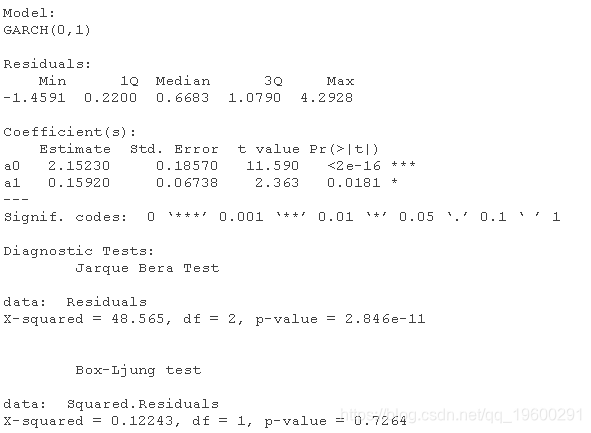
ts(2*fitted.values^2)
plot.ts(hhat)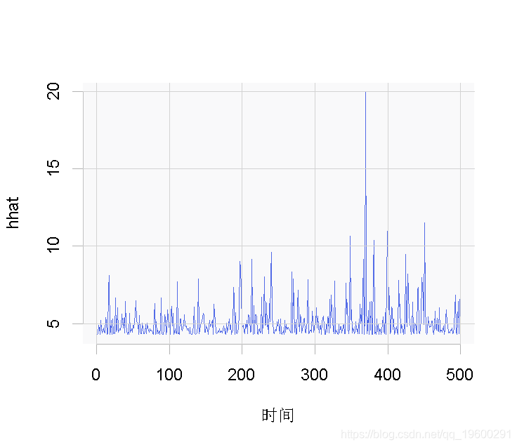
图 对数据集的ARCH(1)方差的估计
GARCH模型
# 使用软件包\`garch\`来建立GARCH模型

fit(spec=garch, data=r)
coef(Fit)
fitted.values
fit$sigma^2)
plot.ts(hhat)
图: 使用数据集的标准GARCH模型(sGARCH)。
# tGARCH

garchfit(spec, data=r, submodel="TGARCH")
coef(garchfit)
fitted.values

fit$sigma^2)
plot.ts(hhat)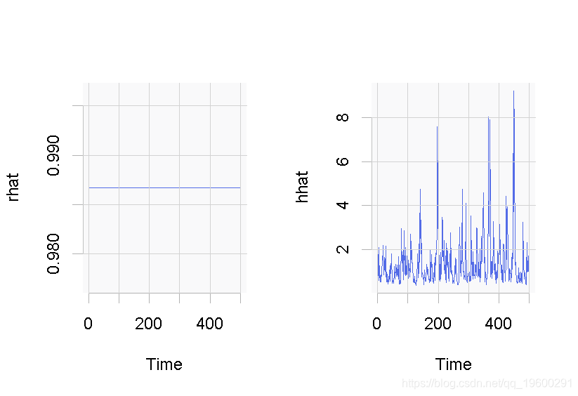
图: 数据集的tGARCH模型
# GARCH-IN-MEAN模型

fit( data=r,
           distribution="std",variance=list(model="fGARCH")
coef(garchFit)
fit$fitted.values
fit$sigma^2)
plot.ts(hhat)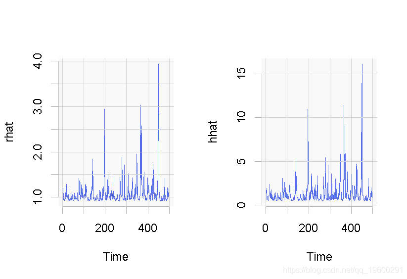
图:使用数据集的GARCH-in-mean模型的一个版本
图显示了GARCH模型的几个版本。预测结果可以通过ugarchboot()来获得。
可下载资源
关于作者
Kaizong Ye是拓端研究室(TRL)的研究员。在此对他对本文所作的贡献表示诚挚感谢,他在上海财经大学完成了统计学专业的硕士学位,专注人工智能领域。擅长Python.Matlab仿真、视觉处理、神经网络、数据分析。
本文借鉴了作者最近为《R语言数据分析挖掘必知必会 》课堂做的准备。
非常感谢您阅读本文,如需帮助请联系我们!
 Python和Lag-Llama金融时序预测收益率零样本与微调对比回测实证研究|附代码数据
 Python、SPSS单指数、FF三因子模型、决策树分析沪深300指数、申万风格指数、10年期国债收益率、300ETF期权波动率指数数据优化金融期货市场预测|附代码数据
 Python实现Transformer神经网络时间序列模型可视化分析商超蔬菜销售数据筛选高销量单品预测|附代码数据
 Python中国证券成分股波动率量化:ARIMA-随机森林预测、MPT投资组合优化、四维评价体系与动态仓位策略