
本文使用R语言进行stan泊松回归Poisson regression。
本文展示了如何使用R语言进行stan泊松回归Poisson regression 的例子。
可下载资源
读取数据
summary(eba1977)
×
R
stan是建立贝叶斯模型的一款软件,可以在R中通过rstan调用。下面是安装rstan的步骤:
(1) 在网页http://cran.r-project.org/bin/windows/Rtools/下载安装最新的Rtools。
(2) 退出当前的R,然后重新启动R。
(3) 在R中运行下述三行程序,检查Rtools是否安装正常。
|
1
2
3
|
Sys.getenv(‘PATH’)
system(‘g++ -v’)
system(‘where make’)
|
(4) 在R中运行下述两行程序,安装rstan:
|
1
2
|
source(‘http://mc-stan.org/rstan/install.R’, echo = TRUE,max.deparse.length = 2000)
install_rstan()
|
(5)rstan安装完成后,重新启动R,就可以进行贝叶斯分析了。
##          city      age         pop             cases
##  Fredericia:6   40-54:4   Min.   : 509.0   Min.   : 2.000
##  Horsens   :6   55-59:4   1st Qu.: 628.0   1st Qu.: 7.000
##  Kolding   :6   60-64:4   Median : 791.0   Median :10.000
##  Vejle     :6   65-69:4   Mean   :1100.3   Mean   : 9.333
##                 70-74:4   3rd Qu.: 954.8   3rd Qu.:11.000
##                 75+  :4   Max.   :3142.0   Max.   :15.000
普通 Poisson model
glm1 <- glm(formula = cases ~ age + city + offset(log(pop)),
            family  = poisson(link = "log"),
            data    = eba1977)
summary(glm1)
##
## Call:
## glm(formula = cases ~ age + city + offset(log(pop)), family = poisson(link = "log"),
## data = eba1977)
##
## Deviance Residuals:
## Min 1Q Median 3Q Max
## -2.63573 -0.67296 -0.03436 0.37258 1.85267
##
## Coefficients:
## Estimate Std. Error z value Pr(>|z|)
## (Intercept) -5.6321 0.2003 -28.125 < 2e-16 ***
## age55-59 1.1010 0.2483 4.434 9.23e-06 ***
## age60-64 1.5186 0.2316 6.556 5.53e-11 ***
## age65-69 1.7677 0.2294 7.704 1.31e-14 ***
## age70-74 1.8569 0.2353 7.891 3.00e-15 ***
## age75+ 1.4197 0.2503 5.672 1.41e-08 ***
## cityHorsens -0.3301 0.1815 -1.818 0.0690 .
## cityKolding -0.3715 0.1878 -1.978 0.0479 *
## cityVejle -0.2723 0.1879 -1.450 0.1472
## ---
## Signif. codes: 0 '***' 0.001 '**' 0.01 '*' 0.05 '.' 0.1 ' ' 1
##
## (Dispersion parameter for poisson family taken to be 1)
##
## Null deviance: 129.908 on 23 degrees of freedom
## Residual deviance: 23.447 on 15 degrees of freedom
## AIC: 137.84
##
## Number of Fisher Scoring iterations: 5视频
R语言中RStan贝叶斯层次模型分析示例
Stan
数据
## 模型矩阵
modMat <- as.data.frame(model.matrix(glm1))
modMat$offset <- log(eba1977$pop)
names(modMat) <- c("intercept", "age55_59", "age60_64", "age65_69", "age70_74",
                   "age75plus", "cityHorsens", "cityKolding", "cityVejle", "offset")

dat   <- as.list(modMat)
dat$y <- eba1977$cases
dat$N <- nrow(modMat)
dat$p <- ncol(modMat) - 1
## 读取Stan文件
fileName <- "./Homework_7KY_poisson.stan"
stan_code <- readChar(fileName, file.info(fileName)$size)
cat(stan_code)## 运行 Stan
resStan <- stan(model_code = stan_code, data = dat,
chains = 3, iter = 3000, warmup = 500, thin = 10)##
## TRANSLATING MODEL 'stan_code' FROM Stan CODE TO C++ CODE NOW.
## COMPILING THE C++ CODE FOR MODEL 'stan_code' NOW.
## In file included from file60814bc1cb78.cpp:8:
## In file included from /Library/Frameworks/R.framework/Versions/3.1/Resources/library/rstan/include//stansrc/stan/model/model_header.hpp:17:
## In file included from /Library/Frameworks/R.framework/Versions/3.1/Resources/library/rstan/include//stansrc/stan/agrad/rev.hpp:5:
## /Library/Frameworks/R.framework/Versions/3.1/Resources/library/rstan/include//stansrc/stan/agrad/rev/chainable.hpp:87:17: warning: 'static' function 'set_zero_all_adjoints' declared in header file should be declared 'static inline' [-Wunneeded-internal-declaration]
## static void set_zero_all_adjoints() {
## ^
## In file included from file60814bc1cb78.cpp:8:
## In file included from /Library/Frameworks/R.framework/Versions/3.1/Resources/library/rstan/include//stansrc/stan/model/model_header.hpp:21:
## /Library/Frameworks/R.framework/Versions/3.1/Resources/library/rstan/include//stansrc/stan/io/dump.hpp:26:14: warning: function 'product' is not needed and will not be emitted [-Wunneeded-internal-declaration]
## size_t product(std::vector<size_t> dims) {
## ^
## 2 warnings generated.
##
## SAMPLING FOR MODEL 'stan_code' NOW (CHAIN 1).
##
## Iteration: 1 / 3000 [ 0%] (Warmup)
## Iteration: 300 / 3000 [ 10%] (Warmup)
## Iteration: 501 / 3000 [ 16%] (Sampling)
## Iteration: 800 / 3000 [ 26%] (Sampling)
## Iteration: 1100 / 3000 [ 36%] (Sampling)
## Iteration: 1400 / 3000 [ 46%] (Sampling)
## Iteration: 1700 / 3000 [ 56%] (Sampling)
## Iteration: 2000 / 3000 [ 66%] (Sampling)
## Iteration: 2300 / 3000 [ 76%] (Sampling)
## Iteration: 2600 / 3000 [ 86%] (Sampling)
## Iteration: 2900 / 3000 [ 96%] (Sampling)
## Iteration: 3000 / 3000 [100%] (Sampling)
## # Elapsed Time: 0.142295 seconds (Warm-up)
## # 0.543612 seconds (Sampling)
## # 0.685907 seconds (Total)
##
##
## SAMPLING FOR MODEL 'stan_code' NOW (CHAIN 2).
##
## Iteration: 1 / 3000 [ 0%] (Warmup)
## Iteration: 300 / 3000 [ 10%] (Warmup)
## Iteration: 501 / 3000 [ 16%] (Sampling)
## Iteration: 800 / 3000 [ 26%] (Sampling)
## Iteration: 1100 / 3000 [ 36%] (Sampling)
## Iteration: 1400 / 3000 [ 46%] (Sampling)
## Iteration: 1700 / 3000 [ 56%] (Sampling)
## Iteration: 2000 / 3000 [ 66%] (Sampling)
## Iteration: 2300 / 3000 [ 76%] (Sampling)
## Iteration: 2600 / 3000 [ 86%] (Sampling)
## Iteration: 2900 / 3000 [ 96%] (Sampling)
## Iteration: 3000 / 3000 [100%] (Sampling)
## # Elapsed Time: 0.13526 seconds (Warm-up)
## # 0.517139 seconds (Sampling)
## # 0.652399 seconds (Total)
##
##
## SAMPLING FOR MODEL 'stan_code' NOW (CHAIN 3).
##
## Iteration: 1 / 3000 [ 0%] (Warmup)
## Iteration: 300 / 3000 [ 10%] (Warmup)
## Iteration: 501 / 3000 [ 16%] (Sampling)
## Iteration: 800 / 3000 [ 26%] (Sampling)
## Iteration: 1100 / 3000 [ 36%] (Sampling)
## Iteration: 1400 / 3000 [ 46%] (Sampling)
## Iteration: 1700 / 3000 [ 56%] (Sampling)
## Iteration: 2000 / 3000 [ 66%] (Sampling)
## Iteration: 2300 / 3000 [ 76%] (Sampling)
## Iteration: 2600 / 3000 [ 86%] (Sampling)
## Iteration: 2900 / 3000 [ 96%] (Sampling)
## Iteration: 3000 / 3000 [100%] (Sampling)
## # Elapsed Time: 0.120931 seconds (Warm-up)
## # 0.509901 seconds (Sampling)
## # 0.630832 seconds (Total)## 绘制轨迹图
traceplot(resStan, pars = c("beta"), inc_warmup = TRUE)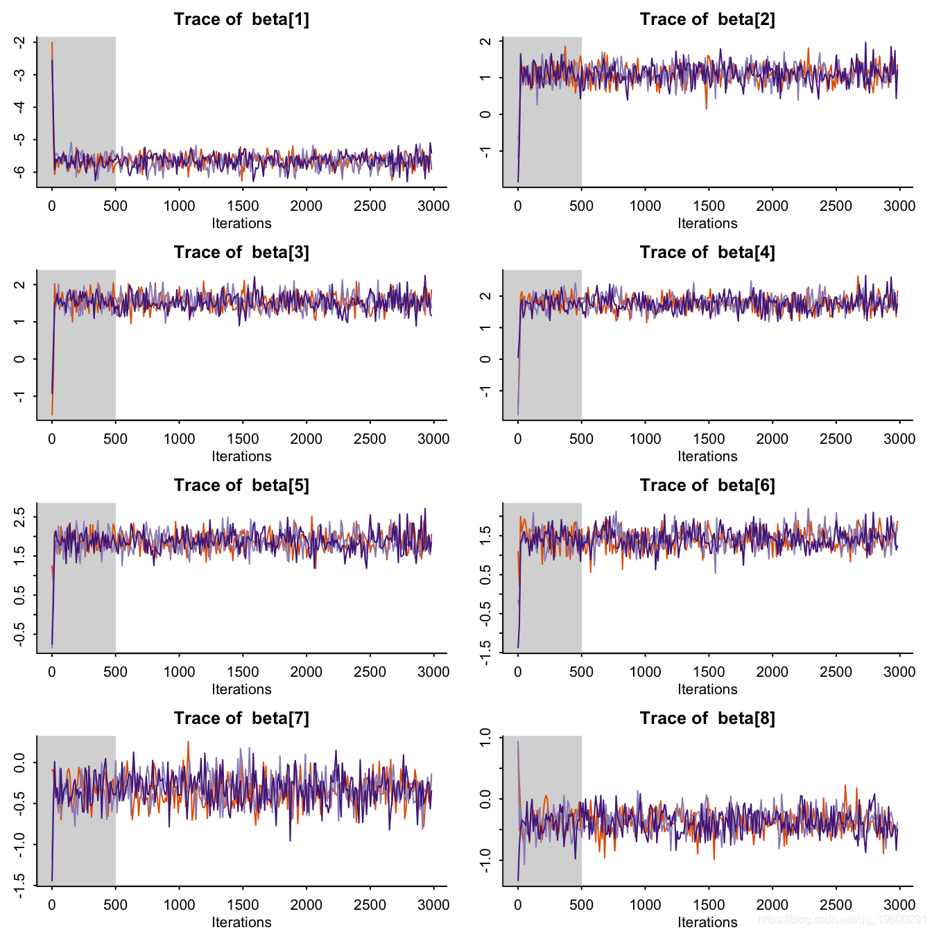
比较
## 模型结果
tableone::ShowRegTable(glm1, exp = FALSE)
## beta [confint] p
## (Intercept) -5.63 [-6.04, -5.26] <0.001
## age55-59 1.10 [0.61, 1.59] <0.001
## age60-64 1.52 [1.07, 1.98] <0.001
## age65-69 1.77 [1.32, 2.22] <0.001
## age70-74 1.86 [1.40, 2.32] <0.001
## age75+ 1.42 [0.93, 1.91] <0.001
## cityHorsens -0.33 [-0.69, 0.03] 0.069
## cityKolding -0.37 [-0.74, -0.00] 0.048
## cityVejle -0.27 [-0.64, 0.09] 0.147## 贝叶斯结果
print(resStan, pars = c("beta"))## Inference for Stan model: stan_code.
## 3 chains, each with iter=3000; warmup=500; thin=10;
## post-warmup draws per chain=250, total post-warmup draws=750.
##
## mean se_mean sd 2.5% 25% 50% 75% 97.5% n_eff Rhat
## beta[1] -5.66 0.01 0.21 -6.13 -5.80 -5.64 -5.51 -5.29 655 1
## beta[2] 1.11 0.01 0.25 0.60 0.95 1.11 1.28 1.60 750 1
## beta[3] 1.53 0.01 0.23 1.10 1.38 1.51 1.68 2.00 750 1
## beta[4] 1.77 0.01 0.25 1.30 1.60 1.76 1.94 2.24 750 1
## beta[5] 1.87 0.01 0.24 1.40 1.71 1.86 2.02 2.37 750 1
## beta[6] 1.42 0.01 0.25 0.94 1.25 1.42 1.58 1.95 631 1
## beta[7] -0.33 0.01 0.18 -0.69 -0.45 -0.32 -0.21 0.03 703 1
## beta[8] -0.37 0.01 0.19 -0.74 -0.50 -0.38 -0.24 -0.01 664 1
## beta[9] -0.28 0.01 0.19 -0.66 -0.40 -0.27 -0.15 0.09 698 1
##
## Samples were drawn using NUTS(diag_e) at Mon Apr 13 21:43:02 2015.
## For each parameter, n_eff is a crude measure of effective sample size,
## and Rhat is the potential scale reduction factor on split chains (at
## convergence, Rhat=1).可下载资源
关于作者
Kaizong Ye是拓端研究室(TRL)的研究员。在此对他对本文所作的贡献表示诚挚感谢,他在上海财经大学完成了统计学专业的硕士学位,专注人工智能领域。擅长Python.Matlab仿真、视觉处理、神经网络、数据分析。
本文借鉴了作者最近为《R语言数据分析挖掘必知必会 》课堂做的准备。
非常感谢您阅读本文,如需帮助请联系我们!
 视频讲解|Stata和R语言自助法Bootstrap结合GARCH对sp500收益率数据分析
 Python谷歌商店Google Play APP评分预测:LASSO、多元线性回归、岭回归模型对比研究
 Python+AI提示词出租车出行轨迹:梯度提升GBR、KNN、LR回归、随机森林融合预测及贝叶斯概率异常检测研究
 Python对Airbnb北京、上海链家租房数据用逻辑回归LR、决策树、岭回归、Lasso、随机森林、XGBoost、神经网络kmeans聚类分析市场影响因素|数据分享