考虑我们从实验、事件等中观察到一些数据 y 的情况。
我们将观察结果 y 解释为某个随机变量 Y 的实现:
统计模型是对未知参数 θ 的 Y 分布的规范。
通常,观测值 y = (y1, . . . , yn) ∈ Rn 是一个向量,而 Y = (Y1, . . . ., Yn) 是一个随机向量。在这种情况下,统计模型是 Y1 联合分布的规范, . . , Yn 直到未知参数 θ。
手机示例
观察示例: yi = 学生 i 在讲座的前 10 分钟内查看他们的手机。
模型:
在许多实验和情况下,观测值 Y1, . . . , Yn 不具有相同的分布。Y1 的分布, 。. . , Yn 可能取决于非随机量 x1, 。. . , xn 称为协变量。
示例:矮小的学生在数学考试中取得更高的分数吗?
Yi = 平均分,xi = 身高
模型:
模型拟合
我们将描述模型拟合的过程如下:
1. 模型规范——指定观测值 Y1, 的分布。. . , Yn 可达未知参数。
2. 模型未知参数的估计。
3. 推理——这涉及构建置信区间和测试关于参数的假设。
4. 诊断——检查模型与数据的拟合程度。
“理想”模型应该
• 与观察到的数据相当吻合。
• 不包含不必要的参数。
• 易于解释。
R中的示例
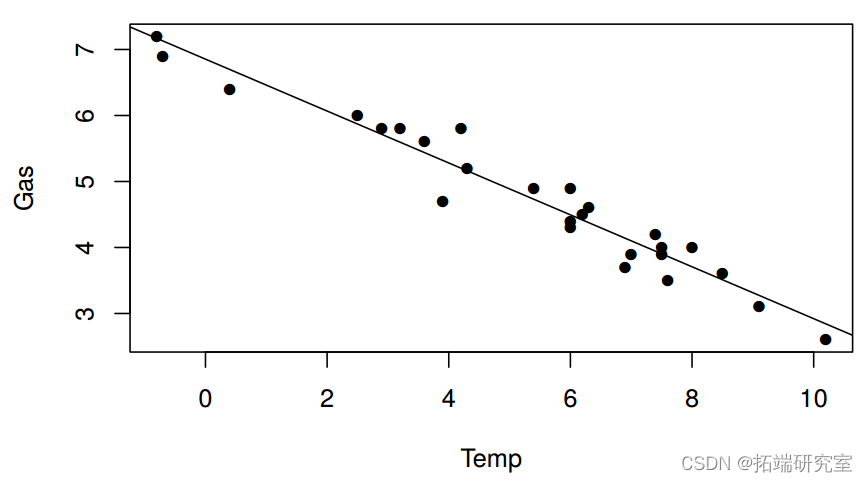
假设我们有由家庭燃气消耗量和平均外部温度组成的数据(见下表)。外部温度可以用来衡量家庭使用的燃气量吗?
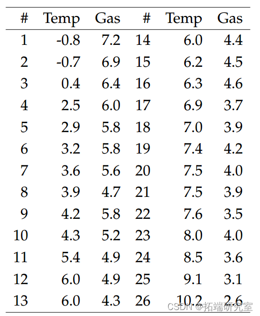
我们将 Gas 作为因变量,Yi 和 Temp 作为协变量 xi。假设我们使用线性正态模型来解释数据;其中 Yi 是独立的 N(µi, σ2),其中 µi = β1 + β2xi 对于 i = 1, . . . , 26. 对于这个模型,我们有
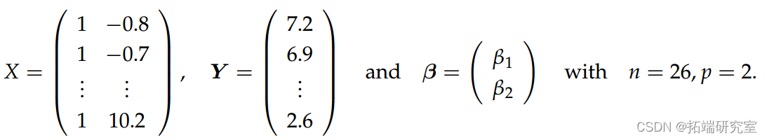
然后计算 MLE 使用以下命令。首先,我们合并观察向量 Y 和设计矩阵 X:
> X <- cbind(1,dat$Temp)
 可以使用以下命令找到:
> qr(t(X)%*%X)$rank

\[1\] 2
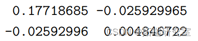
作为 有满秩,我们可以计算它的逆:
> solve(t(X)%*%X)

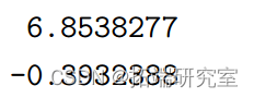
MLE β =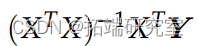 可以计算如下:
> betahat
然后绘制模型拟合我们可以使用
随时关注您喜欢的主题
> lines(x=xs,y=btaht\[1\]+xs*beaht\[2\])
此外,残差平方和 (RSS) 为
> RSS <- t(ehat)%*%ehat

> RSS

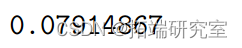
最后,我们可以计算 :
:
> sg2ht <- RSS/(26-2)

> sg2at
诊断
系数
衡量线性模型拟合优度的一种方法是检查决定系数;我们现在解释。在只有截距项的最简单模型中
我们有 RSS = ∑in=1(Yi – Y)2。具有更多参数和大型设计矩阵的较大模型将具有较小的 RSS。
对于包含截距项的模型,线性模型质量的度量是
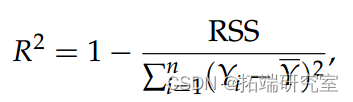
这称为决定系数或 R2 统计量。请注意,0 ≤ R2 ≤ 1 和 R2 = 1 对应于“完美”模型。
异常值
异常值是不符合其余数据的一般模式的观察结果。异常值可能由于数据记录错误、数据是两个或多个总体的混合以及模型需要改进等原因而发生。我们将假设一个满秩的设计矩阵。
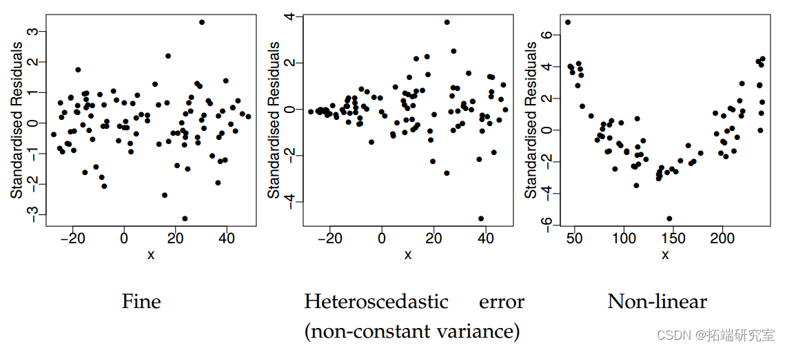
残差图
杠杆
我们可能对每个观察结果对模型拟合的影响程度感兴趣。例如,考虑残差 e 其中
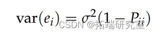
杠杆对应于观察残差的方差。
库克距离
衡量观察影响的另一种方法是考虑它对估计量 β 的变化或影响。一种这样的衡量标准是库克的距离
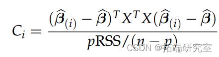
 是不使用第 i 个观测值计算的估计量。经验法则是查看 Ci 接近 1 的观测值。
库克距离的解释
我们现在更详细地研究残差、杠杆和库克距离。考虑下面给出的 4 个人工数据集,每个数据集都安装了正常的线性模型。此外,还显示了残差与杠杆的关系图。
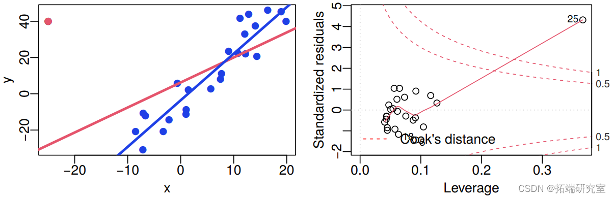
红色数据点是可疑数据点,即高杠杆、高残差(绝对值)或两者兼有。红线是包括红色数据点的拟合,黑线是不包括红色数据点的拟合。
例子
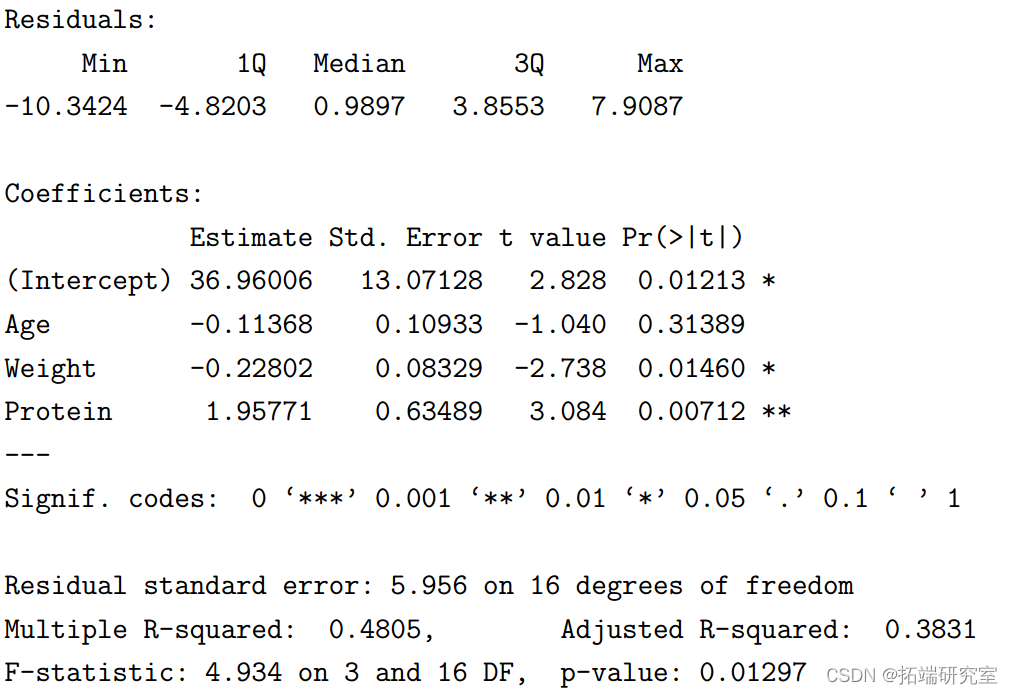
表中的数据显示了 20 名接受高碳水化合物饮食的男性糖尿病患者从复合碳水化合物中获得的总卡路里百分比,以及他们的年龄、体重和卡路里作为蛋白质的百分比。
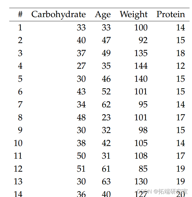
我们将碳水化合物值作为我们的反应 Yi,以年龄、体重和蛋白质作为协变量。然后我们用 Yi ∼ N(µi, σ2) 拟合正态线性模型,其中

然后,要找到 β 的最大似然估计量,我们需要求解 :
:
> beta.hat <- solve(t(X)%*%X)%*%t(X)%*%y

> t(beta.hat)

可以计算方差的无偏估计量 RSS/(n – p),并用于计算每个分量的标准差 .
.
> sqrt(diag(sig.sq.hat\*solve(t(X)%\*%X)))

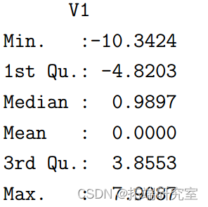
残差是
> summary(ehat)
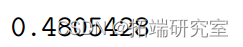
R2 和它的调整版本 R2 系数是
> R2
> 1-(RS/(20-4))/(RS0/(20-1))
我们可以使用 R 中的 lm 函数检查这些结果,如下所示:
> summary(mylm1)
接下来,我们执行单向方差分析测试
> anova(mylm1)
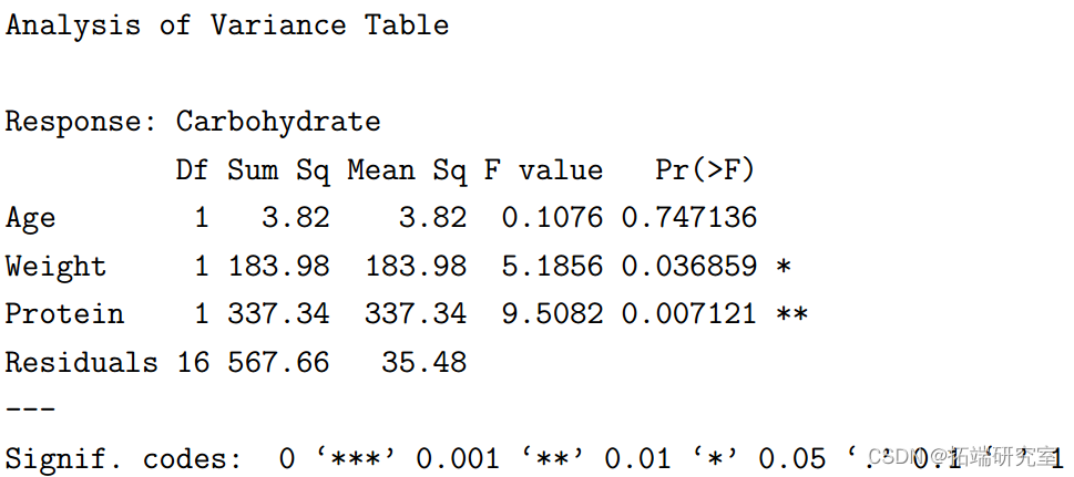
注意输出的形式——即 Sum Sq 是基于上述模型的差异,即
> sum(mym2$esiuls^2)-sum(mym3$reials^2)

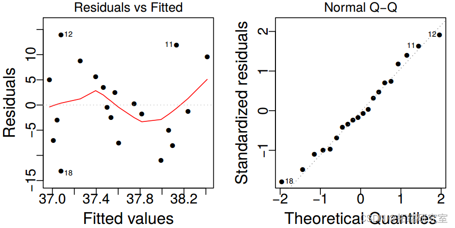
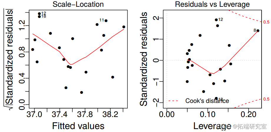
最后,R 还可以为我们生成一些残差图,如下所示:
> plot(mylm2)
自测题
Q1) (a) In R fit the normal linear model with:
Based upon the summary of the model, do you think that the model fits the data well? Explain your reasoning using the values reported in the R summary
(b) Perform a hypothesis test to ascertain whether or not to include the intercept term | use a 5% significance level. Include your code.
(c) Conduct a hypothesis test comparing the models:
E(Y ) = β1 against E(Y ) = β1 + β2×2 + β3×3 + β4×4
as a 5% level. Include your code
(d) By inspecting the leverages and residuals, identify any potential outliers. Name these data points by their index number. Give your reasoning as to why you believe these are potential outliers. You may present up to three plots if necessary.
Q2) We shall now consider a GLM with a Gamma response distribution.
(a) Show that a random variable Y where Y follows a Gamma distribution with probability density function: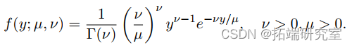
is a member of the exponential family | taking the form a(φ) = φ. State the canonical link function and the variance function in terms of the expected response and the dispersion parameter.
(b) Show that the deviance for a GLM with a Gamma response distribution is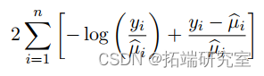
(c) Rewrite (by \hand”) the IWLS algorithm specifically for the Gamma response and using the link:
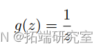
This is called the inverse link function.
(d) Write the components of the total score U1; : : : ; Up and the Fisher information matrix for this model.
(e) Given the observations y, what is a sensible initial guess to begin the IWLS algorithm in general?
(f) Manually write an IWLS algorithm to fit a Gamma GLM using your data, mydat, using the inverse link and same linear predictor in Q1a). Use the deviance as the convergence criteria and initial guess of β as (0:5; 0:5; 0:5; 0:5). Present your code and along with your final estimate of β and final deviance.
(g) Based on your IWLS results, compute φbD and φbp and the estimates of var(βb2). In R fit the model again with a Gamma response i.e.
> glm(y~x1+x2+x3,family=Gamma,data=mydat)
Note the capital G in Gamma. Verify the results with your IWLS results.
(h) Give a prediction for the response given by the model for x1= 13, x2= 5 x3= 0:255
and give a 91% confidence interval for this prediction. Include your code.
(i) Perform a hypothesis test between this model and another model with the same link and response distribution but with linear predictor η where ηi = β1 + β2xi1 + β3xi2 for i = 1; : : : ; n:
Use a 5% significance level. You may use the deviance function here. Include your code.
(j) Using your IWLS results, manually compute the leverages of the observations for this model | present your code (but not the values) and plot the leverages against the observation index number.
(k) Proceed to investigate diagnostic plots for your Gamma GLM. Identify any potential outliers | give your reasoning. Remove the most suspicious data point
| you must remove 1 and only 1 | and refit the same model. Compare and comment on the change of the model with and without this data point | you may wish to refer to the relative change in the estimated coefficients. You may present up to three plots if necessary.
可下载资源
关于作者
Kaizong Ye是拓端研究室(TRL)的研究员。在此对他对本文所作的贡献表示诚挚感谢,他在上海财经大学完成了统计学专业的硕士学位,专注人工智能领域。擅长Python.Matlab仿真、视觉处理、神经网络、数据分析。
本文借鉴了作者最近为《R语言数据分析挖掘必知必会 》课堂做的准备。
非常感谢您阅读本文,如需帮助请联系我们!
 R语言Stan贝叶斯回归置信区间后验分布可视化模型检验
 R语言分类回归分析考研热现象分析与考研意愿价值变现
 SPSS用多元逐步回归模型对上证指数预测、描述统计和相关分析可视化研究
 R语言、WEKA关联规则、决策树、聚类、回归分析工业企业创新情况影响因素数据