
在保险定价中,风险敞口通常用作模型索赔频率的补偿变量。
如果我们必须使用相同的程序,但是一个程序的暴露时间为6个月,而另一个则是一年,那么自然应该假设平均而言,第二个驾驶员的事故要多两倍。
可下载资源
这是使用标准(均匀)泊松过程来建模索赔频率的动机。人们在这里还可以看到法律问题,因为如果(部分)退还保费,则可以按比例进行。风险与暴露成正比。因此,如果 Yi表示被保险人的理赔数量i,则具有特征Xi和风险敞口Ei,通过泊松回归,我们写
或等同
根据该表达式,曝光量的对数是一个解释变量,不应有系数(此处的系数取为1)。我们不能使用暴露作为解释变量吗?我们会得到一个单位参数吗?
当然,在进行费率评估的过程中,这可能不是一个相关的问题,因为精算师需要预测年度索赔频率(因为保险合同应提供一年的保险期)。但是,更好地了解人们为什么会离开我们的投资组合(例如,在任期前取消保险单,或者某天不续签)可能会很有趣。
为了更具体和更好地理解,请考虑以下模型:考虑使用Poisson流程对索赔到达进行建模,以及专职于其保险公司的人员。
> n=983
> D1=as.Date("01/01/1993",'%d/%m/%Y')
> D2=as.Date("31/12/2013",'%d/%m/%Y')


> for(i in 1:n){
+   expo=D2-arrival[i]
+   w=0
+   while(max(w)<expo) w=c(w,max(w)+1+trunc(rexp(1,1/1000)))
+   exposure[i]=departure[i]-arrival[i]
+   N[i]=max(0,length(w)-2)}
> df=data.frame(N=N,E=exposure/365)在这里,两次索赔之间的预期时间为1000天。泊松过程的(年度)强度在这里
> 365/1000
[1] 0.365
因此,如果我们对曝光的对数进行Poisson回归,我们应该获取一个相近参数
> log(365/1000)
[1] -1.007858
在这里,具有偏移量的常数的回归为

> summary(reg)

Call:

Deviance Residuals:
    Min       1Q   Median       3Q      Max
-3.4145  -0.4673   0.2367   0.8770   3.6828

Coefficients:
            Estimate Std. Error z value Pr(>|z|)
(Intercept) -1.04233    0.02532  -41.17   <2e-16 ***
---
Signif. codes:  0 ‘***’ 0.001 ‘**’ 0.01 ‘*’ 0.05 ‘.’ 0.1 ‘ ’ 1

(Dispersion parameter for poisson family taken to be 1)

    Null deviance: 1116.9  on 982  degrees of freedom
Residual deviance: 1116.9  on 982  degrees of freedom
AIC: 3282.9

Number of Fisher Scoring iterations: 5
这与我们刚才所说的一致。如果我们以曝光量的对数作为可能的解释变量进行回归,则我们期望其系数接近1。
Call:

Deviance Residuals:
    Min       1Q   Median       3Q      Max
-3.0810  -0.8373  -0.1493   0.5676   3.9001

Coefficients:
            Estimate Std. Error z value Pr(>|z|)
(Intercept) -1.03350    0.08546  -12.09   <2e-16 ***
log(E)       1.00920    0.03292   30.66   <2e-16 ***
---
Signif. codes:  0 ‘***’ 0.001 ‘**’ 0.01 ‘*’ 0.05 ‘.’ 0.1 ‘ ’ 1

(Dispersion parameter for poisson family taken to be 1)

    Null deviance: 2553.6  on 982  degrees of freedom
Residual deviance: 1064.2  on 981  degrees of freedom
AIC: 3762.7

Number of Fisher Scoring iterations: 5
如果我们保留偏移量并添加变量,我们可以看到它变得无用(对单位参数的测试)
Call:


Deviance Residuals:
    Min       1Q   Median       3Q      Max
-3.0810  -0.8373  -0.1493   0.5676   3.9001

Coefficients:
             Estimate Std. Error z value Pr(>|z|)
(Intercept) -1.033503   0.085460 -12.093   <2e-16 ***
log(E)       0.009201   0.032920   0.279     0.78
---
Signif. codes:  0 ‘***’ 0.001 ‘**’ 0.01 ‘*’ 0.05 ‘.’ 0.1 ‘ ’ 1

(Dispersion parameter for poisson family taken to be 1)

    Null deviance: 1064.3  on 982  degrees of freedom
Residual deviance: 1064.2  on 981  degrees of freedom
AIC: 3762.7

Number of Fisher Scoring iterations: 5
在这里,我们确实具有纯泊松过程,因此曝光至关重要,因为泊松分布的参数与曝光成正比。但是我们不能从曝光中学到其他东西。
考虑一些真实数据。
  nocontrat exposition zone puissance agevehicule
1        27       0.87    C         7           0
2       115       0.72    D         5           0
3       121       0.05    C         6           0
4       142       0.90    C        10          10
5       155       0.12    C         7           0
6       186       0.83    C         5           0
  ageconducteur bonus marque carburant densite region nbre
1            56    50     12         D      93     13    0
2            45    50     12         E      54     13    0
3            37    55     12         D      11     13    0
4            42    50     12         D      93     13    0
5            59    50     12         E      73     13    0
6            75    50     12         E      42     13    0
如果考虑暴露的对数的泊松回归,将会得到什么?
> summary(reg)

Call:

Deviance Residuals:
    Min       1Q   Median       3Q      Max
-0.3988  -0.3388  -0.2786  -0.1981  12.9036

Coefficients:
                Estimate Std. Error z value Pr(>|z|)
(Intercept)     -2.83045    0.02822 -100.31   <2e-16 ***
log(exposition)  0.53950    0.02905   18.57   <2e-16 ***
---
Signif. codes:  0 ‘***’ 0.001 ‘**’ 0.01 ‘*’ 0.05 ‘.’ 0.1 ‘ ’ 1

(Dispersion parameter for poisson family taken to be 1)

    Null deviance: 12931  on 49999  degrees of freedom
Residual deviance: 12475  on 49998  degrees of freedom
AIC: 16150

Number of Fisher Scoring iterations: 6
如果将曝光量添加到偏移量中,会发生什么情况?(我们使用非参数转换,可视化发生的情况)
plot(reg,se=TRUE)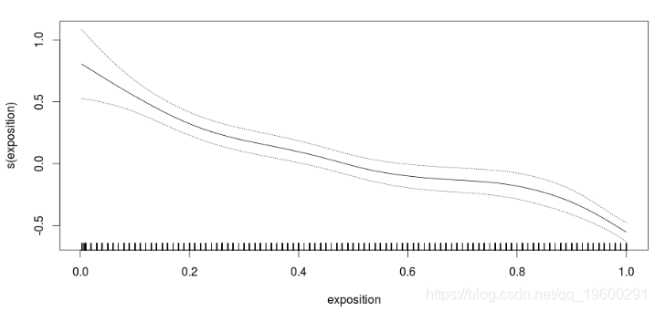
有明显而显着的效果。时间越长,他们获得索赔的可能性就越小。实际上,无需进行回归即可观察到它。
> plot(h1$mids,h1$density,type='s',lwd=2,col="red")
> lines(h0$mids,h0$density,type='s',col='blue',lwd=2)
蓝色为没有索赔人的风险密度,红色为有一个或多个索赔人的风险密度。
因此,在这里,我们不能假设参数的单位值。这意味着什么 ?我们可以重现这种行为吗?
为了更好地理解被保险人,请考虑两种可能的行为。第一个是:如果公司在没有索赔的几年后没有提供大幅折扣,则被保险人可能会离开公司。例如,如果被保险人在5年内没有索偿,那么5年后,他将离开公司(例如,获得更高的价格)。该代码
> df=data.frame(N=N,E=exposure/365)如果我考虑的是1500天而不是5年。
> summary(reg)

Call:

Deviance Residuals:
    Min       1Q   Median       3Q      Max
-1.5684  -0.9668  -0.2321   0.4244   3.6265

Coefficients:
            Estimate Std. Error z value Pr(>|z|)
(Intercept) -2.50844    0.10286  -24.39   <2e-16 ***
log(E)       1.65738    0.04494   36.88   <2e-16 ***
---
Signif. codes:  0 ‘***’ 0.001 ‘**’ 0.01 ‘*’ 0.05 ‘.’ 0.1 ‘ ’ 1

(Dispersion parameter for poisson family taken to be 1)

    Null deviance: 2567.31  on 982  degrees of freedom
Residual deviance:  885.71  on 981  degrees of freedom
此处,系数(明显)大于1。
> summary(reg)

Call:

Deviance Residuals:
    Min       1Q   Median       3Q      Max
-1.5684  -0.9668  -0.2321   0.4244   3.6265

Coefficients:
            Estimate Std. Error z value Pr(>|z|)
(Intercept) -2.50844    0.10286  -24.39   <2e-16 ***
log(E)       0.65738    0.04494   14.63   <2e-16 ***
---
Signif. codes:  0 ‘***’ 0.001 ‘**’ 0.01 ‘*’ 0.05 ‘.’ 0.1 ‘ ’ 1

(Dispersion parameter for poisson family taken to be 1)

    Null deviance: 1114.24  on 982  degrees of freedom
Residual deviance:  885.71  on 981  degrees of freedom
AIC: 2897.9
这里显然存在偏见:长时间待在办公室的人更可能发生事故。这与我们的想法一致,因为客户的风险较低。
第二种行为是:有时,被保险人对索赔的处理方式不满意,他们可能会在第一次索赔后离开。考虑一种情况,在一项索赔之后,被保险人很可能(例如,概率为50%)离开公司。与其假设被保险人不喜欢理赔管理,不如考虑汽车被严重损坏以至于他不能再开车了。因此,支付保险费将毫无用处。这里的代码
> for(i in 1:n){
+   expo=D2-arrival[i]
+   w=0


+   exposure[i]=departure[i]-arrival[i]}
> df=data.frame(N=N,E=exposure/365)
在这里,在每次索赔之后,被保险人扔硬币查看他是否取消合同。
Deviance Residuals:
     Min        1Q    Median        3Q       Max
-2.28402  -0.47763  -0.08215   0.33819   2.37628

Coefficients:
            Estimate Std. Error z value Pr(>|z|)
(Intercept)  0.09920    0.04251   2.334   0.0196 *
log(E)       0.30640    0.02511  12.203   <2e-16 ***
---
Signif. codes:  0 ‘***’ 0.001 ‘**’ 0.01 ‘*’ 0.05 ‘.’ 0.1 ‘ ’ 1

(Dispersion parameter for poisson family taken to be 1)

    Null deviance: 666.92  on 982  degrees of freedom
Residual deviance: 498.29  on 981  degrees of freedom
AIC: 2666.3
这次,参数(再次显着)小于1。
Deviance Residuals:
     Min        1Q    Median        3Q       Max
-2.28402  -0.47763  -0.08215   0.33819   2.37628

Coefficients:
            Estimate Std. Error z value Pr(>|z|)
(Intercept)  0.09920    0.04251   2.334   0.0196 *
log(E)      -0.69360    0.02511 -27.625   <2e-16 ***
---
Signif. codes:  0 ‘***’ 0.001 ‘**’ 0.01 ‘*’ 0.05 ‘.’ 0.1 ‘ ’ 1

(Dispersion parameter for poisson family taken to be 1)

    Null deviance: 1116.87  on 982  degrees of freedom
Residual deviance:  498.29  on 981  degrees of freedom
AIC: 2666.3
现在的情况已经大不相同了,因为那些待久的人应该不会遇到很多离开的机会。显然,他们没有太多要求。如果某人的风险敞口很大,那么上面输出中的负号表示该人平均应该没有太多债权。
如我们所见,这些模型产生了相当大的差异输出。注意,可能有更多的解释。例如,根据提取数据的方式,
- 在过去的二十年中,所有遵守的政策,
- 到现在为止所有在特定日期生效的政策
- 在某个特定日期生效的所有政策,直到之后的一年
- 现在生效的所有政策
到目前为止,我们一直在使用第一种方法,但是其他方法会产生不同的解释。
 【视频】N-Gram、逻辑回归反欺诈模型文本分析招聘网站欺诈可视化|附数据代码
 R语言Stan贝叶斯回归置信区间后验分布可视化模型检验
 R语言分类回归分析考研热现象分析与考研意愿价值变现
 【专题】2024商业健康险与医药协同创新模式研究报告合集PDF分享(附原数据表)