如果_真实_模型包括_X_ 1 和_X_ 2 ,但我们忘记了_X_ 2,那么 – 在某些情况下 – 对_X_的估计将会有偏差。OVB 需要:cor( X 1, X 2)!= 0 和 cor( X 1, y ) != 0
同方差性
为了做出有效的推断,我们假设误差方差是恒定的 – 如果不是,我们冒着做出错误推断的风险(没有偏差,只影响 SE,补救措施:稳健的 SE)
可下载资源
内生性
如果_X_影响_Y_但_Y_也影响_X_,则我们具有内生性,这将导致估计量有偏。
虚拟变量和交互
虚拟变量
可以取两个值的变量,例如分数(小班、大班),也称为指示变量或二元变量。
当我们估计这个模型时会发生什么?
值_i_ = β 0 + β 1大_i_ + ε _i_
y__i = β_0 + _β_1_d__i + ε__i
小班的估计是多少?
大班的估计是多少?

示例:学校数据
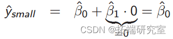
小班的期望分数是多少?
◦ β^0
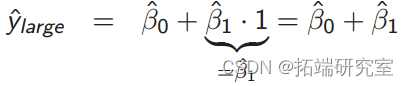
大班的预期分数是多少?
◦ β^0 + β^1 •
小班和大班之间的期望差异是什么?
◦ β^1
> summary(mol.mll)

虚拟变量与回归
当我们将虚拟变量添加到具有连续解释变量的模型时会发生什么?
y__i = β_0 + _β_1_x__i + ε__i
y__i = β_0 + _β_1_x__i + β_2_d + ε__i
如果大班_d_ = 1,小班_d_ = 0,我们得到大班:
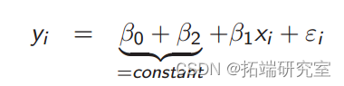
对于小班,我们得到这个:
插图
学校数据
> del <- lm(tetcr ~ Sraio + igscol, data=dt1)

> summary(me2)
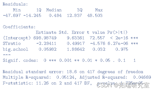

一个学生对每个老师的边际效应是多少?
βSTR比
大班有什么影响?
◦ β ^大班.__学校
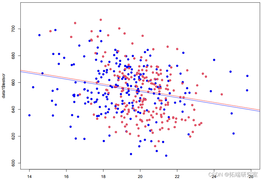
STratio 对小班/大班的影响是否相同?
◦是的,_β_ _^ STratio_对任何区都是相同的(平行线)
随时关注您喜欢的主题
添加虚拟变量可以改变一切
交互项
回归模型
在多元回归模型中, β ^1 描述了__X 1的边际效应,_同时控制_了_X_ 2 的效应。
内置假设_X_ 1 对所有观测值具有相同的效应。
交互
放宽这种假设的一种方法是允许效果变化。
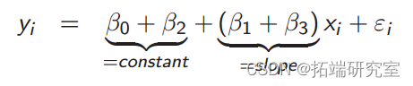
我们通过使用交互来实现这一点,我们将解释变量的乘积添加到模型中:
Y__i = β_0 + _β_1_X_1_i + β_2_X_2_i + β_3_X_1_i · X_2_i + ε__i
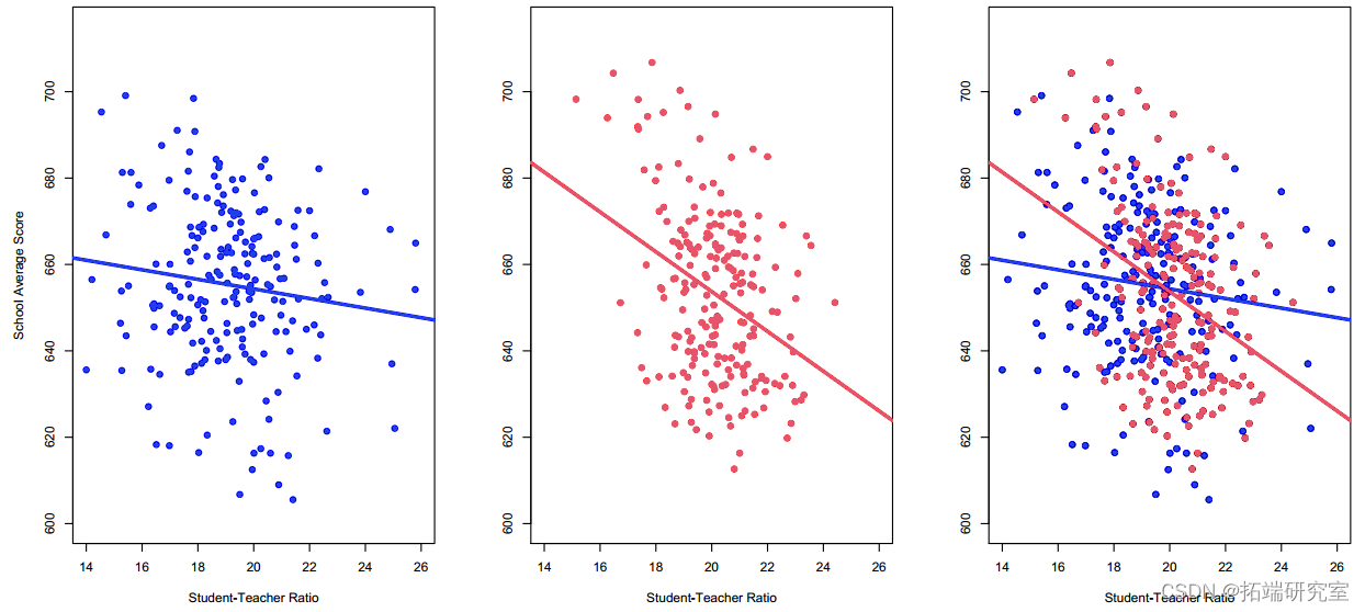
图 1
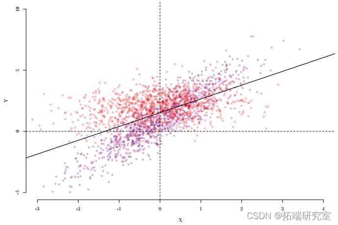
图 2
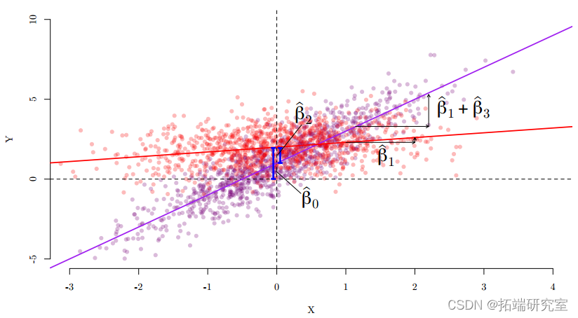
图 3
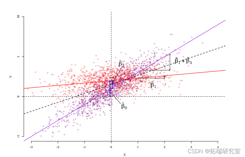
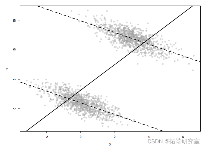
交互:虚拟变量和回归
- 为什么假设效应 ( β 1 ) 在所有子组中都是恒定的?
- 让我们根据 big.school 让 STratio 产生不同的效果:
y__i = β_0 + _β_1_x__i + β_2_d__i + β_3_d__i · x__i + ε__i
如果大班_d_ = 1,小班_d_ = 0,我们得到大班:
对于小班:

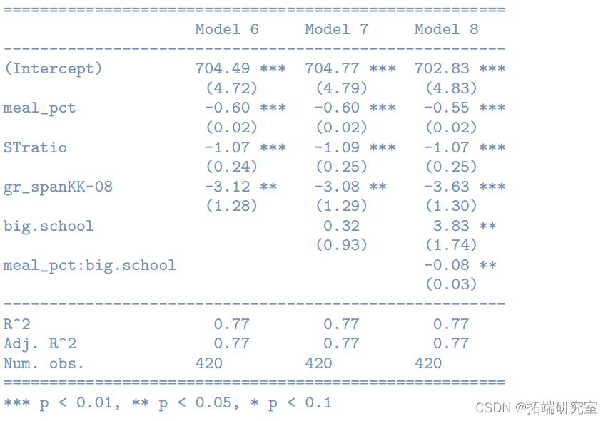
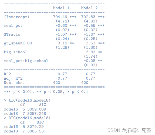
> srereg(list(model1,model2, model3))
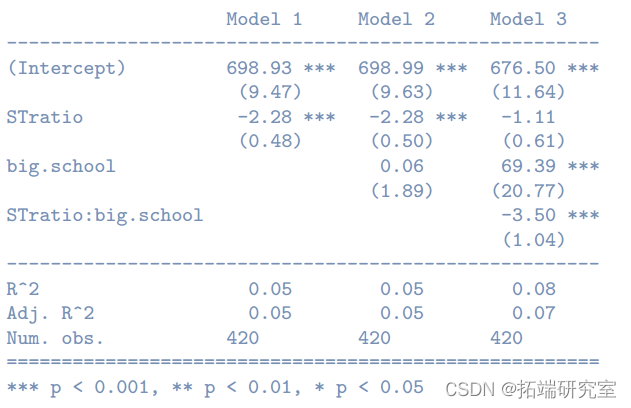
STratio & 大班
虚拟变量可以做什么
定性信息
我们可以将定性信息(名义变量)纳入回归模型
允许灵活模型
我们可以使用与虚拟变量的交互作用来允许不同子组中 X 的不同边际效应。
交互作用:_x_和_x_ 2
为什么要加_x_ 2?
有时我们希望_x_对_y_的影响是非线性的。
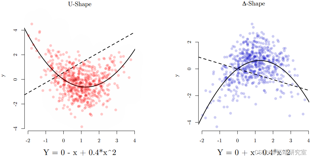
交互作用:_x_和_x_2
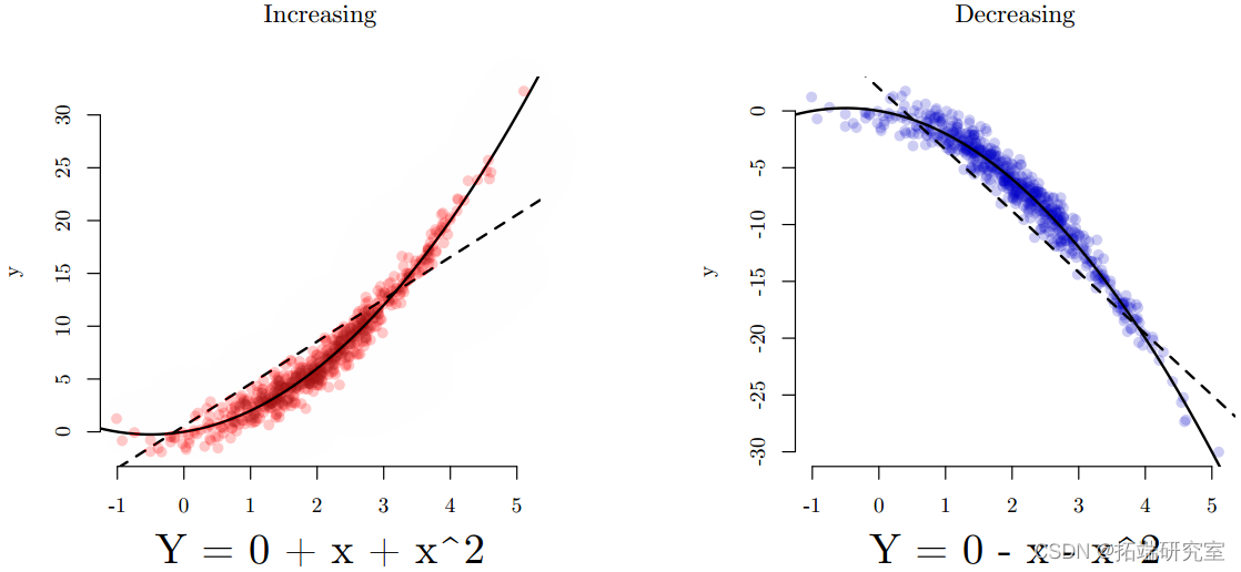
如果所有_Xi_ > 0:
- 如果_β_ x_为正且_β _x_ 2为负,则得到倒 U 形•如果_β_ x_为负且_β _x_ 2为正,则得到 u 形
- 如果两者都是正面/负面的,你会得到:
让我们看看大班
> screreg(list(model4, model5))

让我们看看大班
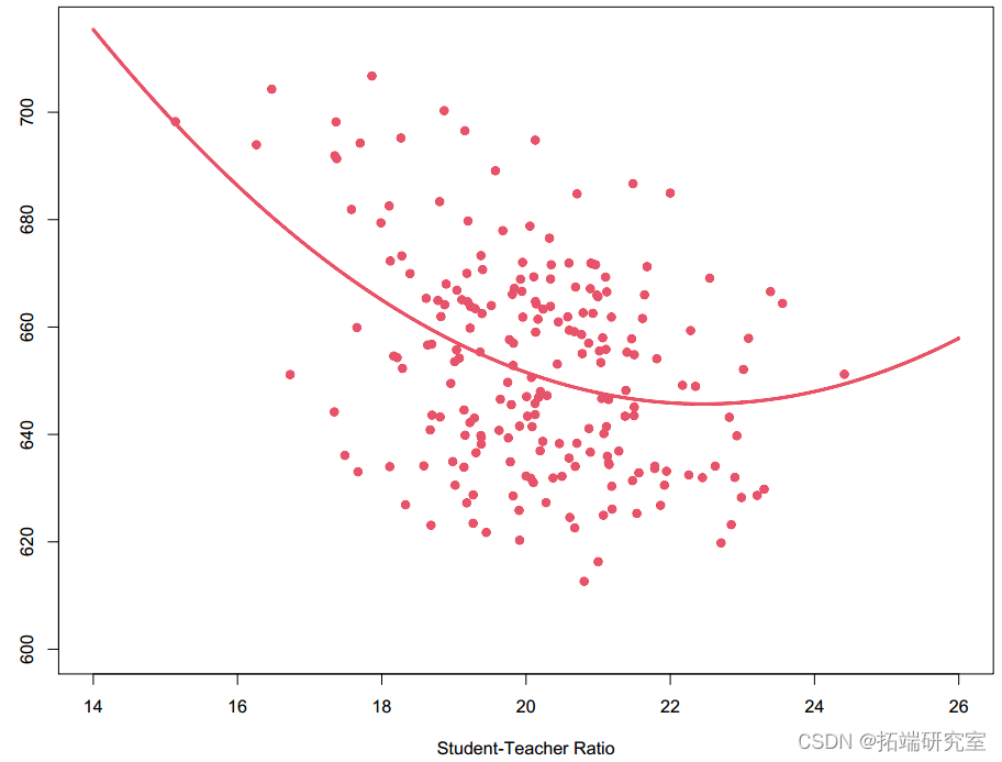
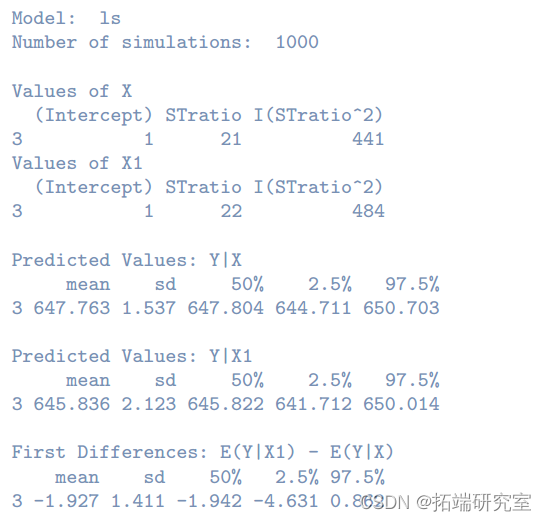
_X_的作用是什么?
由于包含 X 2 项,X 增加一个单位的影响将不再具有恒定的影响。这被称为第一个差异。
解,x = 14
> s.u <- sim(zout, x=xlow,1=x.hih)

> summary(.ot)
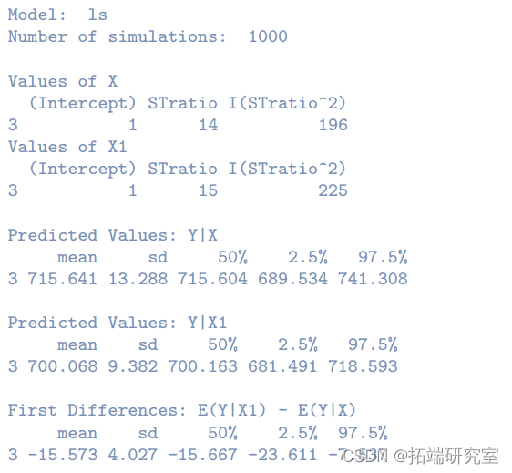
现在 x = 21
> xow <- set(zt,STratio=21)

> x.igh <- stx(z.t,STratio=22)
交互作用的后果
• 效果很难从输出中立即判断(正面或负面)
• 边际效应不是恒定的 – 任何关于效果的陈述都取决于 x 值
联合假设检验
相互测试模型
区分模型
我们有许多测试来评估数据是否更适合模型 A 或 B。
• F 检验:告诉您哪个模型具有更好的数据拟合。
• AIC:告诉您哪个模型更适合,非常类似于 F 检验
• BIC:类似于 AIC,但对复杂性进行惩罚
!AIC 和 BIC 是特殊的,因为这两个模型不需要相互嵌套。在相同的样本上估计它们就足够了。
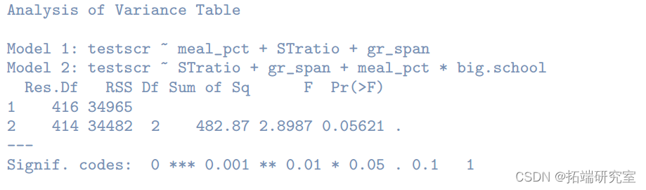
F-Test:学校规模重要吗?
> senrg(list(model6,model7,model8),str = c(0.01,0.05,0.1))
> anova
=========================================================================
OLS 输出中的 F 检验
模型 1:
模型 2: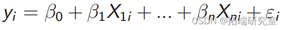
> summary(model6)

相互测试模型
为什么要惩罚复杂性?
模型越复杂,对数据的拟合就越好。
更复杂,更少简约。由于过度拟合数据的危险,我们需要简约的模型进行预测。
理论检验与预测
当我们通过检验假设的方式检验理论时,我们使用F 检验。
在进行预测时,我们希望使用 BIC 来区分模型。
AIC 和 BIC
Akaike 信息准则和贝叶斯信息准则
AIC 和 BIC 都反映了数据拟合的程度以及包含的解释变量的数量(复杂性)。当数据拟合更好时,度量会下降 。当添加更多变量时,度量会上升,较低的值更好。
• 在试图区分两个模型时,BIC 和 AIC 可能会给出相互矛盾的建议
• 如果您正在测试一个理论,如果模型是嵌套的,则使用 F 检验,否则使用 AIC
• 如果您正在进行预测,请使用 AIC 或 BIC
◦ 越保守度量是 BIC
F 检验:示例
• 请记住:F 检验拒绝了更简约的模型
• AIC 几乎不支持更复杂的模型(3059.089>3057.248)
• BIC 拒绝了更复杂的模型
screeg(list(mode6,mol8),stars = c(0.01,0.05,0.1))
F 检验、AIC 和 BIC
• 使用 F 检验时:
◦ 一个模型必须嵌套在另一个模型中
◦ 两个模型都必须根据相同的观测值进行估计
• AIC 和 BIC 可以处理未嵌套的模型
• AIC 和 BIC 仅在两个模型在同一样本上估计时才有效
自测题
A politician argues that immigrant children (defined as children for whom English is not their first language) cause entire districts to perform badly on standardized tests. Use the California school data to verify if there is any relationship between share of immigrant children and average test score.
There is a measure for how CME or LME a country is (market index=0 is fully CME, 1 is fully LME). The theory predicts that being close to either ideal type should cause lower unemployment rates due to consistent institutional arrangements. Create a model to test this statement and include at least three additional explanatory variables. Interpret the results statistically and substantially
Estimate a model explaining why somebody self-identifies as left or right on a 1-10 scale. Use at least two variables and in addition age. Is age a significant factor? Interpret st & su. In a second step, control for party affiliation and verify whether the results from the original model change or still hold
Datasets
1) SwissData2011.dta
Post-referendum survey among people living in Switzerland. The following list of variables is your
codebook:
• VoteYes { Is 1 if someone voted yes and is 0 if someone voted no.
• male { Is 1 for men and 0 for women.
• age { Age in years.
• LeftRight { Left-Right self placement where low values indicate that a respondent is more to the
left.
• GovTrust { Variable indicates a respondent’s trust in government. Little or no trust is -1, neither
YES nor NO is 0, and +1 if somebody trusts the government.
• ReligFreq { How frequently does a respondent attend a religious service? Never (0), only on special
occasions (1), several times a year (2), once a month (3), and once a week (4).
• university { Binary indicator (dummy) whether respondent has a university degree (1) or not (0).
• party { Indicates which party a respondent supports. Liberals (1), Christian Democrats (2), Social
Democrats (3), Conservative Right (4), and Greens (5).
• income { Income measured in ten different brackets (higher values indicate higher income). You
may assume that this variable is interval-scaled.
• german { Binary indicator (dummy) whether respondent’s mother tongue is German (1) or not
(0)
• suburb { Binary indicator (dummy) whether respondent lives in a suburban neighborhood (1) or
not (0)
• urban { Binary indicator (dummy) whether respondent lives in a city (1) or not (0)
• cars { Number of cars the respondent’s household owns.
• old voter { Variable indicating whether a respondent is older than 60 years (1) or not (0).
• cantonnr { Variable indicating in which of the 26 Swiss cantons a respondent lives.
• nodenomination { Share of citizens in a canton which do not have a denomination.
• urbanization { Share of citizens in a canton which live in urban areas.
2) \violence data v2.dta”
Cross-national data set covering the years from 1980 to 1997.
• code { Country code, alpha, 3-digit
• country { Country name
• africa { Dummy variable for Sub-Saharan African countries. (According to World Bank definition)
• agovdem80 { Anti-government demonstrations: Any peaceful public gathering of at least 100
people.
• assass80 { Assassinations: Number of assassinations per thousand population, decade average.
• blck80 { Black Market Premium: Log of 1+ black market premium, decade average.
• cabchg80 { Major Cabinet Changes: The number of times in a year that a new premier is named.
• compolt80 { Dummy =1 for countries with genocidal incident involving political victims.
• constchg80 { Major Constitutional Changes: The number of basic alternations in a state’s constitution.
• corrupti { Knack and Keefer measure of corruption (1980-89)
• coups80 { Coups d’Etat: The number of extraconstitutional or forced changes in the top government.
• deathsPC80 { Deaths from Political Violence per One Million Citizens
• democ80 { Measure of democracy (Gastil’s Political Rights)
• elf60 { Index of ethnolinguistic fractionalization, 1960. Measures probability that two randomly
drawn individuals come from the same ethno-linguistic group.
• govtcris80 { Major Government Crises: Any rapidly developing situation that threatens to bring
government down.
• gunn1 { Gunnemark1: Percent of population not speaking the official language.
• gunn2 { Gunnemark2: Percent of population not speaking the most widely used language.
• gyp80 { Growth rate of real per capita GDP.
• latinca { Dummy variable for Latin Amercia and the Carribean.
• lly80 { Financial Depth: Ratio of liquid liabilities of the financial system to GDP, dec
• lrgdp80 { Log of initial Income: Log of real per capita GDP measured at the start of each decade.
• lrgdpsq80 { Log of initial (Income squared): Log of Initial real per capita GDP squared.
• lschool80 { Log of Schooling: Log of 1 + average years of school attainment.
• ltelpw80 { Log of Telephones per worker: Log of telephones per 1000 workers
• muller { Probability of two randomly selected individuals speaking different languages.
• newspaperPC80 { Newspapers per capita
• pavroad80 { Paved Roads (percent of total)
• pop80 { Country Population
• purges80 { Purges: Any systematic elimination by jailing or execution of political opposition.
• racialt { Racial tension for 1984, 1 (low tension) to 6 (high tension)
• radiosPC80 { Radios per thousand population
• revols80 { Revolutions: Any illegal or forced change in the top governmental elite.
• riots80 { Riots: Any violent demonstration or clash of more than 100 citizens.
• roberts { Probability that two randomly selected individuals do not speak the same language.
• rulelaw80 { Rule of Law: Law and order tradition (0-6 scale)
• surp80 Fiscal Surplus/GDP: Decade average of ratio of central government surplus (+) to expenditure (-).
• tvPC80 { Televisions per thousand population
• war80 { Dummy for war on national territory during the decade
• warciv80 { Dummy for civil war
• wdiinfmt80 { Infant Mortality Rate:Number of deaths of infants under one year old per 1000
births.
• wdilabag80 { Labor force in farming/forestry/hunting/fishing as a percent of total labor force.
• wditfert80 { Fertility: The average number of children born alive to a woman in her lifetime.
3) WDIdata.csv
Variable descriptions and definitions are available in the WDIdata Description.csv file. This file is
available together with the exam datasets
Question 1
This question consists of three parts (a, b, c) and you must answer all three parts. Use the dataset SwissData2011.dta and answer all parts of the question. You are hired as a political
consultant by a Swiss political party and they ask you to write a report on left-right selfidentification in the Swiss electorate.
a) Provide mean and median for age and left-right self-identification, respectively.
b) Using a t-test you should answer the following question: Are German-speaking voters
more to the right than non-German speaking voters?
c) Using a t-test you should answer the following question: Are older people more to the
right than younger people? Note: use variable old voter.
Question 2
This question consists of three parts (a, b, c) and you must answer all three parts. Use the
dataset \violence data v2.dta” and answer all parts of the question. A widely acknowledged
measure for the extent of poverty is the child mortality rate (wdiinfmt80). Your task is to build
a statistical model explaining child mortality rates.
a) Find at least six theoretically important predictors in the supplied dataset and explain
why you would expect them to have an effect on wdiinfmt80. Estimate a linear regression
model and present your findings. Interpret your findings substantively and statistically.
You should also discuss the model quality. (Note: Do not use latinca or africa in your
model.)
b) Add two dummy variables for Africa and Latin America (africa, latinca) to your model
from part (a) in Question 2. Does the inclusion of these two variables change any of
your findings? Explain how one can statistically test whether these two variables should
be included in the model. Implement your suggested test, present and interpret the test
results. Explain how the inclusion of africa and latinca may help you deal with the omitted
variable bias problem.
c) Civil wars unleash a number of negative consequences and one of them can be wide-spread
poverty. In this third part you will analyze why wars occur. You should develop a logit
model to explain why a country experienced a civil war (warciv80). Estimate the model
and include at least four reasonable explanatory variables (no need to justify your choice,
but make sure that one variable is continuous). Assess the quality of your model by
looking at the correct predictions of civil wars from your model. Provide substantive and
statistical interpretations of the effects and provide at least one figure to illustrate the key
insight of your model.
Question 3
This question consists of four parts (a, b, c, d) and you must answer all four parts. Natural
resource wealth is often associated with poor socio-economic outcomes. This is the so-called
\resource curse” hypothesis that is most often associated with a working paper by Sachs &
Warner (1995) which was further developed in their 2001 article: \Natural Resources and
Economic Development: The curse of natural resources,” European Economic Review 45: 827-
838. Three main elements in the \curse” are negative effects of natural resource wealth on (1)
economic growth, (2) risk of conflict, and (3) political regime type. The original research paper
relied on a cross-sectional design. You’ve been hired by a think tank to produce a report on the
empirical evidence for the resource curse hypothesis using panel data. Furthermore, original
article used a general concept of natural resources. It can be argued that natural resources
differ in their impact on economic growth. For example, the effect of oil abundance may be
more pronounced than the effect of natural gas abundance. In extension of the original Sachs &
Warner argument your contract with the think tank states that you need to empirically assess
whether resource curse is detrimental to economic growth and whether various types of natural
resources have a differential effect on economic growth.
For the exercise we prepared a sample of data from World Bank Development Indicators
(WDI) WDIdata.csv. Please note that WDI variables may differ from variables used in the
original study. Instead you should choose variables for your model conceptually based on your
interpretation of the Sachs & Warner theory and any other readings you may have encountered. For the natural resource wealth, WDI provides data on rents received by the state from
specific natural resources as a percentage of GDP. You may find variable description in the
WDIdata Description.csv file.
Please note that some variables may have unequal coverage across countries and years as
some of the data may be missing. That means that depending on your choice of the variables
you may end up with a smaller effective estimation sample size than expected.
In your analysis you need to address the following questions:
a) Estimate the effect of resource curse on GDP growth rates for the full panel of countries
and years. You should estimate individual, time, and twoway fixed effects models. Explain
how your results change across these three models, and why that may be the case.
You should estimate your model using the relevant R packages as discussed in class and
present model results in a minimally formatted table as specified in the exam description.
b) Explain how you would address the issue of serial correlation in your data. Implement both
approaches that we covered in class { heteroskedasticity and autocorrelation consistent
(HAC) standard errors and lagged dependent variable (LDV) { and discuss your findings.
For the model with lagged dependent variable (LDV) also calculate immediate and longterm effects of natural resources on GDP growth.
You should estimate your model using the relevant R packages as discussed in class and
present model results in a minimally formatted table as specified in the exam description.
In addition, you need to show your calculations of the immediate (short-term) and longterm effects of natural resources on GDP growth.
c) Explain how you would address the issue of cross-sectional dependence. Implement the
Driscoll-Kraay estimator (SCC estimator) to address cross-sectional dependence and explain your results. Please note that depending on the sparsity of your data (how much
of the data is missing) the test for cross-sectional dependence may not have the expected
performance.
可下载资源
关于作者
Kaizong Ye是拓端研究室(TRL)的研究员。在此对他对本文所作的贡献表示诚挚感谢,他在上海财经大学完成了统计学专业的硕士学位,专注人工智能领域。擅长Python.Matlab仿真、视觉处理、神经网络、数据分析。
本文借鉴了作者最近为《R语言数据分析挖掘必知必会 》课堂做的准备。
非常感谢您阅读本文,如需帮助请联系我们!
 【视频】N-Gram、逻辑回归反欺诈模型文本分析招聘网站欺诈可视化|附数据代码
 R语言Stan贝叶斯回归置信区间后验分布可视化模型检验
 R语言分类回归分析考研热现象分析与考研意愿价值变现
 SPSS用多元逐步回归模型对上证指数预测、描述统计和相关分析可视化研究