
分段回归( piecewise regression ),顾名思义,回归式是“分段”拟合的。
其灵活用于响应变量随自变量值的改变而存在多种响应状态的情况,二者间难以通过一种回归模型预测或解释时,不妨根据响应状态找到合适的断点位置,然后将自变量划分为有限的区间,并在不同区间内分别构建回归描述二者关系。
分段回归最简单最常见的类型就是分段线性回归( piecewise linear regression ),即各分段内的局部回归均为线性回归。
可下载资源
本文我们试图预测车辆的制动距离,同时考虑到车辆的速度。
例如在生态学研究中,经常涉及到生态阈值的问题。群落物种多样性或功能模式响应环境特征而改变,但这种响应并不是线性的,生态过程的突然变化可能发生在其中。在某环境梯度范围内,呈现出一种稳定的响应状态;但到达某特定的临界阈值后,可能伴随着剧烈的波动而出现另一种状态的响应。显然在该环境临界点两侧的不同梯度范围内,体现了不同的生态过程,如果在整个环境梯度内使用一种模型描述物种多样性或功能随环境的响应,或许不如分段描述更贴切。
时间尺度上也常应用分段回归描述问题。例如,季节变迁、生态破坏或恢复、物种进化或变异、群落演替等过程中,时而出现某时间点突变的生态过程。这种时间梯度上的突变过程可以是有规律的,如水稻不同生长阶段中,对水分的需求以及各种养分的汲取也大不相同,水稻田的土壤呼吸、物质循环、土壤或根系微生物群落组成或功能等在短期内可能呈现不同模式。也可以是偶然的突发事件,如在严重破坏性的森林大火前后,森林生态系统的物种多样性和功能显然是两种不同的状态。
> summary(reg)

Call:

Residuals:
    Min      1Q  Median      3Q     Max
-29.069  -9.525  -2.272   9.215  43.201

Coefficients:
            Estimate Std. Error t value Pr(>|t|)
(Intercept) -17.5791     6.7584  -2.601   0.0123 *
speed         3.9324     0.4155   9.464 1.49e-12 ***
---
Signif. codes:  0 ‘***’ 0.001 ‘**’ 0.01 ‘*’ 0.05 ‘.’ 0.1 ‘ ’ 1

Residual standard error: 15.38 on 48 degrees of freedom
Multiple R-squared:  0.6511,    Adjusted R-squared:  0.6438
F-statistic: 89.57 on 1 and 48 DF,  p-value: 1.49e-12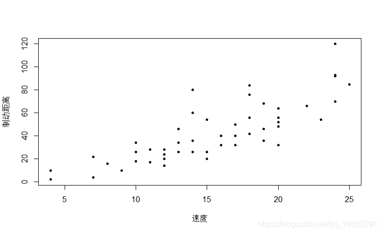
要手动进行多个预测,可以使用以下代码(循环允许对多个值进行预测)
for(x in seq(3,30)){

+ Yx=b0+b1*x
+ V=vcov(reg)
+ IC1=Yx+c(-1,+1)*1.96*sqrt(Vx)
+ s=summary(reg)$sigma
+ IC2=Yx+c(-1,+1)*1.96*s 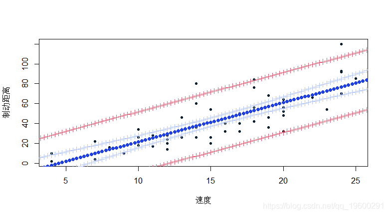
然后在一个随机选择的20个观测值的基础上进行线性回归。
lm(dist~speed,data=cars[I,])目的是使观测值的数量对回归质量的影响可视化。
 Residuals:
    Min      1Q  Median      3Q     Max
-23.529  -7.998  -5.394  11.634  39.348

Coefficients:
            Estimate Std. Error t value Pr(>|t|)
(Intercept) -20.7408     9.4639  -2.192   0.0418 *
speed         4.2247     0.6129   6.893 1.91e-06 ***
---
Signif. codes:  0 ‘***’ 0.001 ‘**’ 0.01 ‘*’ 0.05 ‘.’ 0.1 ‘ ’ 1

Residual standard error: 16.62 on 18 degrees of freedom
Multiple R-squared:  0.7252,    Adjusted R-squared:   0.71
F-statistic: 47.51 on 1 and 18 DF,  p-value: 1.91e-06

> for(x in seq(3,30,by=.25)){

+   Yx=b0+b1*x
+   V=vcov(reg)
+   IC=Yx+c(-1,+1)*1.96*sqrt(Vx)
+ points(x,Yx,pch=19 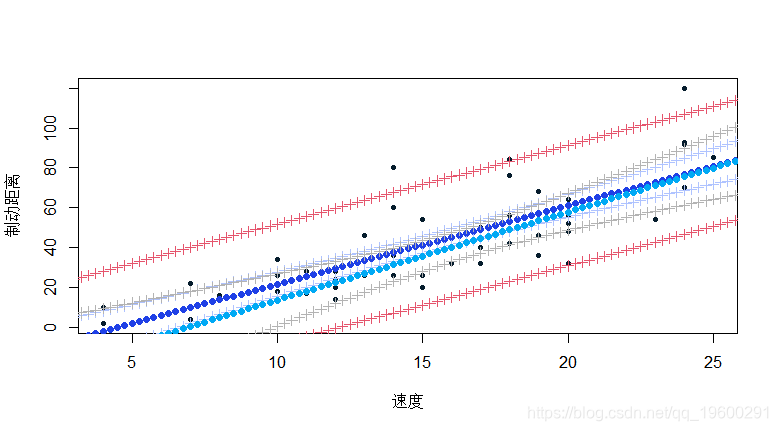
可以使用R函数进行预测,具有置信区间
fit lwr upr
1 42.62976 34.75450 50.50502
2 84.87677 68.92746 100.82607
> predict(reg,
fit lwr upr
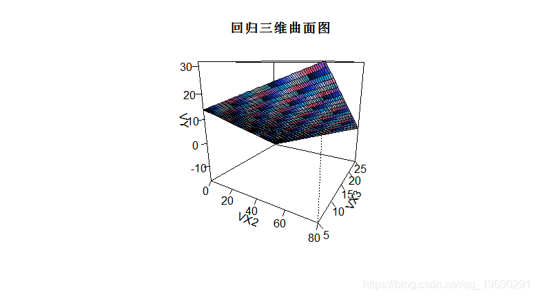
1 42.62976 6.836077 78.42344当有多个解释变量时,“可视化”回归就变得更加复杂了
 > image(VX2,VX3,VY)
> contour(VX2,VX3,VY,add=TRUE)
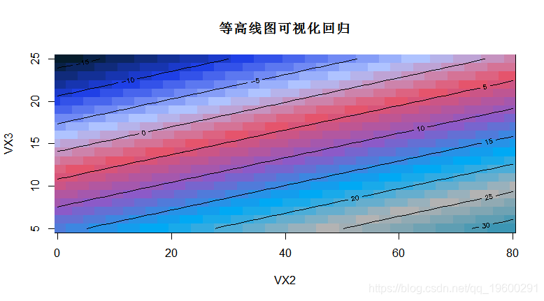
这是一个回归三维曲面_图_
> persp(VX2,VX3,VY,ticktype=detailed)随时关注您喜欢的主题
我们将更详细地讨论这一点,但从这个线性模型中可以很容易地进行非线性回归。我们从距离对数的线性模型开始
> abline(reg1)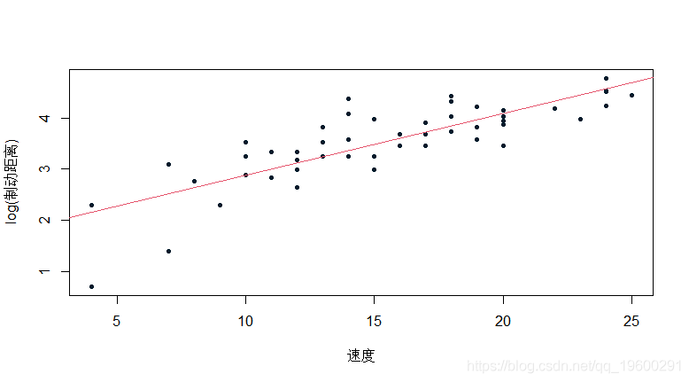
因为我们在这里没有任何关于距离的预测,只是关于它的对数……但我们稍后会讨论它。
lm(sqrt(dist)~speed,data=cars) 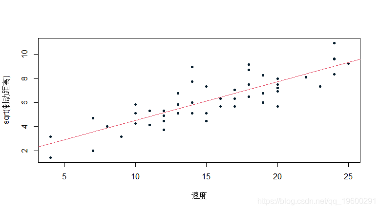
还可以转换解释变量。你可以设置断点(阈值)。我们从一个指示变量开始
 Residuals:
    Min      1Q  Median      3Q     Max
-29.472  -9.559  -2.088   7.456  44.412

Coefficients:
                 Estimate Std. Error t value Pr(>|t|)
(Intercept)      -17.2964     6.7709  -2.555   0.0139 *
speed              4.3140     0.5762   7.487  1.5e-09 ***
speed > s TRUE  -7.5116     7.8511  -0.957   0.3436
---
Signif. codes:  0 ‘***’ 0.001 ‘**’ 0.01 ‘*’ 0.05 ‘.’ 0.1 ‘ ’ 1

Residual standard error: 15.39 on 47 degrees of freedom
Multiple R-squared:  0.6577,    Adjusted R-squared:  0.6432
F-statistic: 45.16 on 2 and 47 DF,  p-value: 1.141e-11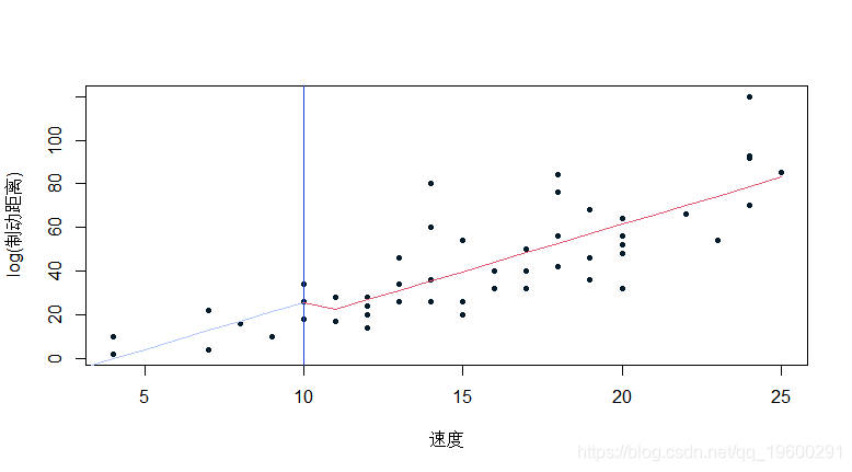
但是你也可以把函数放在一个分段的线性模型里,同时保持连续性。
 Residuals:
    Min      1Q  Median      3Q     Max
-29.502  -9.513  -2.413   5.195  45.391

Coefficients:
                    Estimate Std. Error t value Pr(>|t|)
(Intercept)          -7.6519    10.6254  -0.720  0.47500
speed                 3.0186     0.8627   3.499  0.00103 **
speed - s  1.7562     1.4551   1.207  0.23350
---
Signif. codes:  0 ‘***’ 0.001 ‘**’ 0.01 ‘*’ 0.05 ‘.’ 0.1 ‘ ’ 1

Residual standard error: 15.31 on 47 degrees of freedom
Multiple R-squared:  0.6616,    Adjusted R-squared:  0.6472
F-statistic: 45.94 on 2 and 47 DF,  p-value: 8.761e-12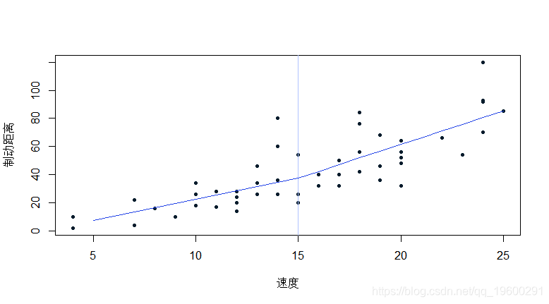
在这里,我们可以想象几个分段
posi=function(x) ifelse(x>0,x,0)


Coefficients:
                     Estimate Std. Error t value Pr(>|t|)
(Intercept)           -7.6305    16.2941  -0.468   0.6418
speed                  3.0630     1.8238   1.679   0.0998 .
positive(speed - s1)   0.2087     2.2453   0.093   0.9263
positive(speed - s2)   4.2812     2.2843   1.874   0.0673 .
---
Signif. codes:  0 ‘***’ 0.001 ‘**’ 0.01 ‘*’ 0.05 ‘.’ 0.1 ‘ ’ 1

Residual standard error: 15 on 46 degrees of freedom
Multiple R-squared:  0.6821,    Adjusted R-squared:  0.6613
F-statistic: 32.89 on 3 and 46 DF,  p-value: 1.643e-11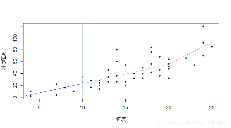
正如目前所看到的,后两个系数的显著性测试并不意味着斜率为零,而是与左侧区域(在两个阈值之前)的斜率显著不同。
 【视频】N-Gram、逻辑回归反欺诈模型文本分析招聘网站欺诈可视化|附数据代码
 R语言Stan贝叶斯回归置信区间后验分布可视化模型检验
 数据分享|R语言Python机器学习预测4案例合集:众筹平台、机票折扣、糖尿病患者、员工满意度