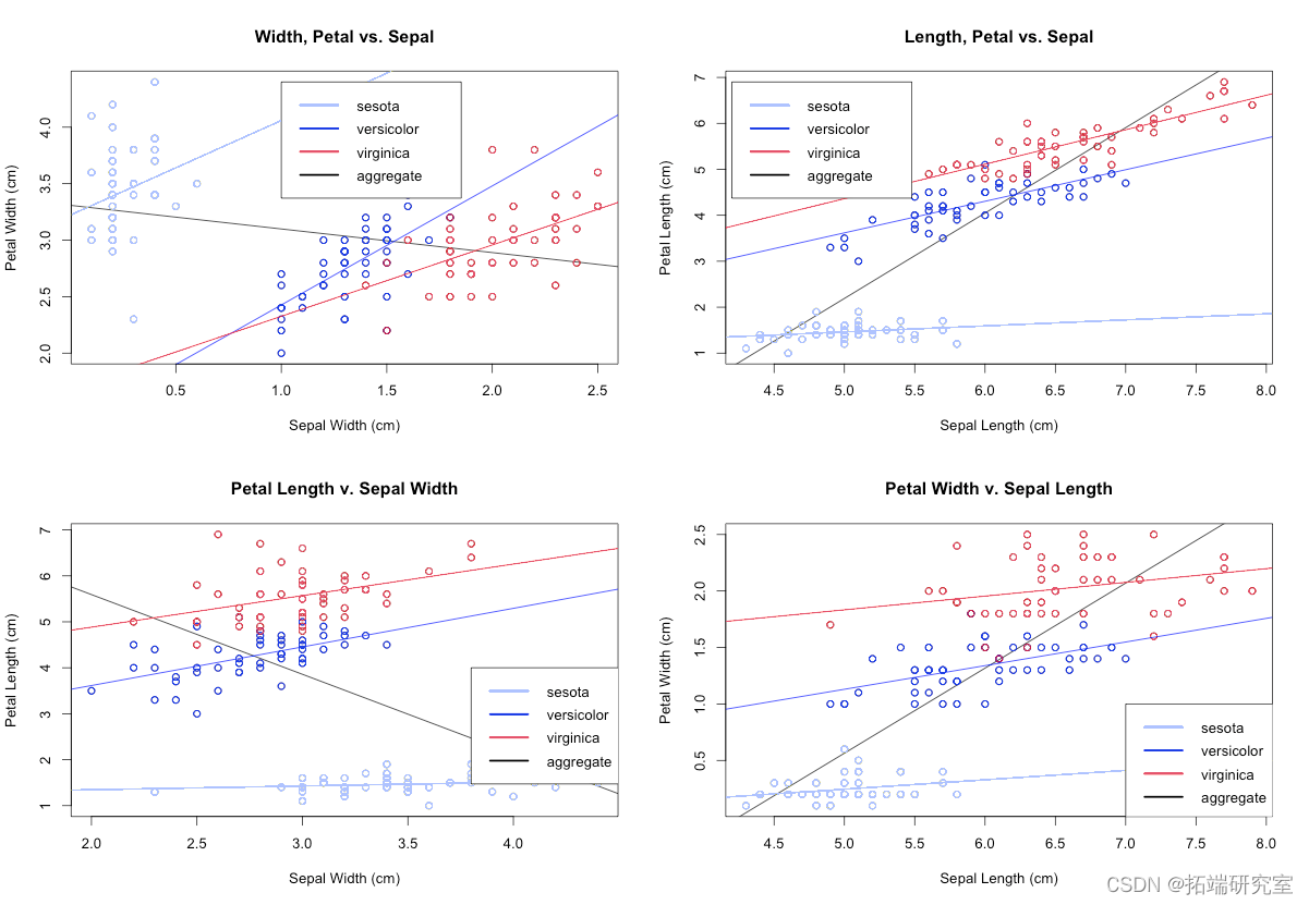
本文将探讨 Fisher 和 Anderson 鸢尾花数据集中呈现的三个变量之间的关系,特别是virginica 和 versicolor 级别的因变量变量物种对预测变量花瓣长度和花瓣宽度的逻辑回归。
单因素方差分析和数据可视化都确定了因变量的一个因素水平,即 I. setosa,很容易与其他两个因素线性分离,具有非常明显的均值和方差,因此不是我们对逻辑回归感兴趣。
介绍
对鸢尾花数据的初步查看引发了关于数据集本身性质的直接问题:为什么要收集如此简单的数据,事实上,我们最初的直觉之一是想知道,鉴于数据集中的信息,是否有可能在进行相关分析和诊断后,建立一个能够对新观察结果进行分类的模型。
我们很惊讶也很高兴得知数据集通常是为了这个目的而采集的。
它最常见的用途是机器学习,特别是分类和模式识别应用。我们开始使用到目前为止所学的工具检查部分数据——即,我们将使用逻辑回归和两种鸢尾花,Virginica 和 versicolor(分别表示为π =0 和π=1)。第三种物种 I. setosa 被排除在外,因为它在所有维度上都与其他两个物种高度分离。
方法
在这种情况下,逻辑回归比卡方或 Fisher 精确检验更合适,因为我们有一个二元因变量和多个预测变量,它还允许我们在控制其他变量的同时清楚地量化各种影响的强度(即每个参数的优势比)。
plot(predicresiduals(logit.fylab="

rl=lm(resi.fit)~bs(predict(.fit),8))

#rl=loess(repredictit.fit))

y=pree=TRUE)

segments(predict(l
结果
创建了一个逻辑模型,一般模型和参数特征如下:

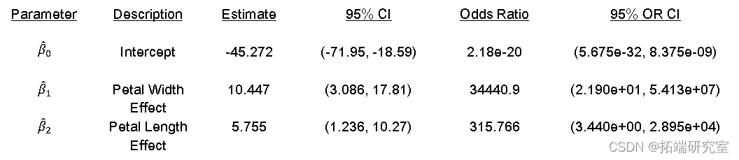
通过查看它们的优势比,可以有效地总结参数估计的含义。显然,截距项并不是特别有趣,因为数据点 (0,0) 在理论上是不可能的,而且远远超出了我们收集的数据范围。β1的优势比![]() 和β2
和β2![]() 更有趣;它们分别代表相关变量的每一个增量,而另一个保持不变时,特定植物属于 I. virginica 物种的几率增加。在这种情况下,很明显,增加花瓣宽度会对特定植物被归类为 I. virginica 的几率产生巨大影响——这种影响大约是花瓣长度的 110 倍。然而,优势比 95% 置信区间都不包含 1,因此我们可以得出结论,这两种效应都具有统计学意义。
更有趣;它们分别代表相关变量的每一个增量,而另一个保持不变时,特定植物属于 I. virginica 物种的几率增加。在这种情况下,很明显,增加花瓣宽度会对特定植物被归类为 I. virginica 的几率产生巨大影响——这种影响大约是花瓣长度的 110 倍。然而,优势比 95% 置信区间都不包含 1,因此我们可以得出结论,这两种效应都具有统计学意义。
library(ggplot2)


#绘图数据

qplot(Petal.Width, Petal.Length, colour = Species,  data = irises, main = "Iris classification")
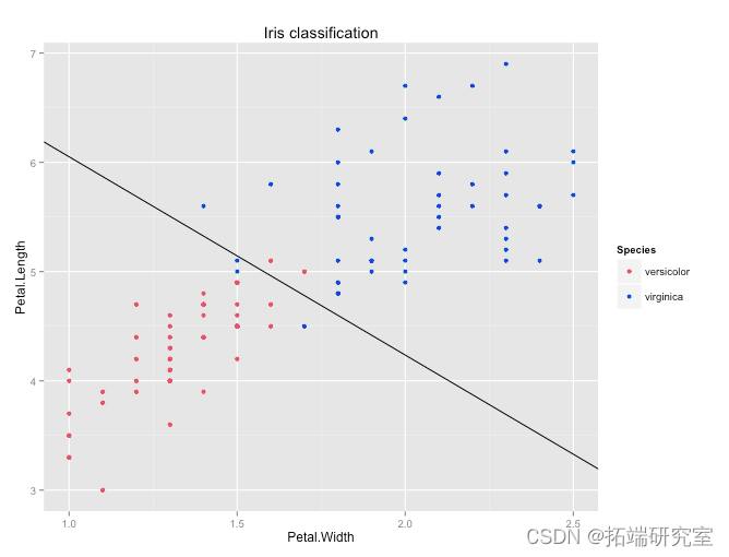

使用模型中的系数估计,我们可以确定一个标准——一个线性判别式——通过它我们可以最好地分离数据。线性判别式的准确度在以下混淆矩阵中给出:
# 从模型中获得预测结果

logit.predictions <- ifelse(predict(logit.fit) > 0,'virginica', 'versicolor')


# 混淆矩阵

table(irises[,5],logit.predictions)

随时关注您喜欢的主题
诊断
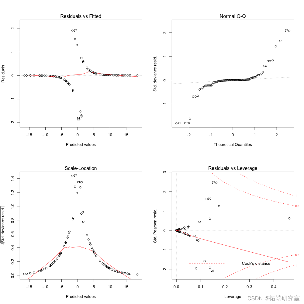
通过检查残差和数据的影响,我们确定了几个潜在的异常观察结果:
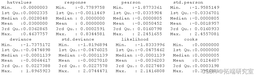
在所有可能有问题的观察中,我们注意到第 57 个观察样本可能是异常点。检查诊断图,我们看到逻辑回归的趋势特征,包括残差与预测图中的两条不同曲线。第 57 个观察样本出现在每个诊断图中,但幸运的是没有超过库克的距离。
结论与讨论
在这种情况下,逻辑模型的使用具有启发性,因为它显示了根据多个预测变量将数据分类为二元因变量技术的强大功能。该模型可预见地显示出最大的不确定性,即在给定维度(即一个物种的数据与另一个物种的数据之间的边界)中观测值接近平均值时。考虑模型是否可以改进,或者不同的模型是否更适合数据是很有趣的;也许对于这个分类问题,k-最近邻方法是必要的。无论如何,6% 的错误分类率实际上是相当不错的;更多的数据肯定会提高这个数字。
自测题
Diagnosis of Depression in Primary Care
To study factors related to the diagnosis of depression in primary care, 400 patients were randomly selected and the following variables were recorded:
DAV: Diagnosis of depression in any visit during one year of care.
0 = Not diagnosed
1 = Diagnosed
PCS: Physical component of SF-36 measuring health status of the patient.
MCS: Mental component of SF-36 measuring health status of the patient
BECK: The Beck depression score.
PGEND: Patient gender
0 = Female
1 = Male
AGE: Patient’s age in years.
EDUCAT: Number of years of formal schooling.
The response variable is DAV (0 not diagnosed, 1 diagnosed), and it is recorded in the first column of the data. The data are stored in the file final.dat and is available from the course web site. Perform a multiple logistic regression analysis of this data using SAS or any other statistical packages. This includes
estimation, hypothesis testing, model selection, residual analysis and diagnostics. Explain your findings in a 3 to 4- page report. Your report may include the following sections:
• Introduction: Statement of the problem.
• Material and Methods: Description of the data and methods that you used for the analysis.
• Results: Explain the results of your analysis in detail. You may cut and paste some of your computer
outputs and refer to them in the explanation of your results.
• Conclusion and Discussion: Highlight the main findings and discuss.
Please cut and paste the computer outputs to your report and do not include any direct computer output as an attachment
Please note that you have also the option of using a similar data set in your own field of interest.
可下载资源
关于作者
Kaizong Ye是拓端研究室(TRL)的研究员。在此对他对本文所作的贡献表示诚挚感谢,他在上海财经大学完成了统计学专业的硕士学位,专注人工智能领域。擅长Python.Matlab仿真、视觉处理、神经网络、数据分析。
本文借鉴了作者最近为《R语言数据分析挖掘必知必会 》课堂做的准备。
非常感谢您阅读本文,如需帮助请联系我们!
 R语言Stan贝叶斯回归置信区间后验分布可视化模型检验
 R语言分类回归分析考研热现象分析与考研意愿价值变现
 R语言逻辑回归logistic模型ROC曲线可视化分析2例:麻醉剂用量影响、汽车购买行为
 R语言逻辑回归、GAM、LDA、KNN、PCA主成分分析分类预测房价及交叉验证