介绍
有限混合模型在应用于数据时非常有用,其中观察来自不同的群体,并且群体隶属关系未知。
模拟数据
首先,我们将模拟一些数据。让我们模拟两个正态分布 – 一个平均值为0,另一个平均值为50,两者的标准差为5。
m1 <- 0
m2 <- 50
sd1 <- sd2 <- 5
N1 <- 100
N2 <- 10

a <- rnorm(n=N1, mean=m1, sd=sd1)
b <- rnorm(n=N2, mean=m2, sd=sd2)
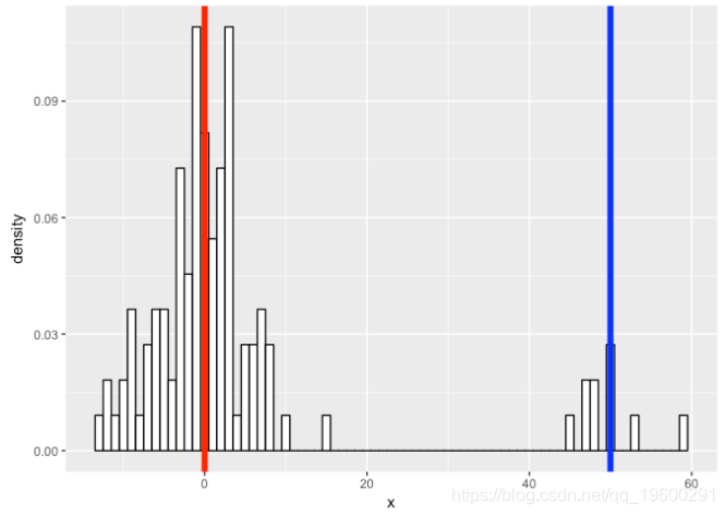
现在让我们将数据“混合”在一起……

print(table(clusters(flexfit), data$class))
##
##       1   2
##   1 100   0
##   2   0  10
参数怎么样?
cat('pred:', c1[1], '\n')
cat('true:', m1, '\n\n')
cat('pred:', c1[2], '\n')
cat('true:', sd1, '\n\n')

cat('pred:', c2[1], '\n')
cat('true:', m2, '\n\n')
cat('pred:', c2[2], '\n')
cat('true:', sd2, '\n\n')
## pred: -0.5613484
## true: 0
##
## pred: 4.799484
## true: 5
##
## pred: 52.86911
## true: 50
##
## pred: 6.89413
## true: 5
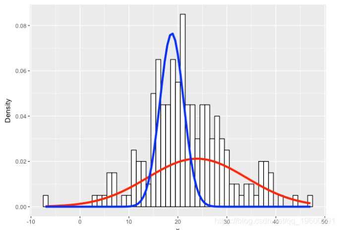
让我们可视化真实数据和我们拟合的混合模型。
ggplot(data) +
geom_histogram(aes(x, ..density..), binwidth = 1, colour = "black", fill = "white") +
stat_function(geom = "line", fun = plot_mix_comps,
                args = list(c1[1], c1[2], lam[1]/sum(lam)),
 stat_function(geom = "line", fun = plot_mix_comps,
                args = list(c2[1], c2[2], lam[2]/sum(lam)),
                colour = "blue", lwd = 1.5) +
ylab("Density")
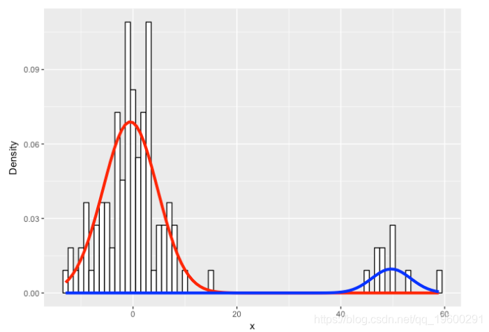

看起来我们做得很好!


例子
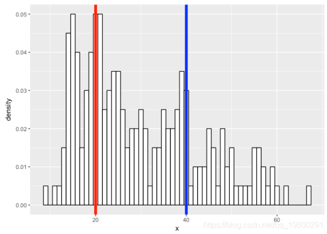
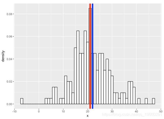
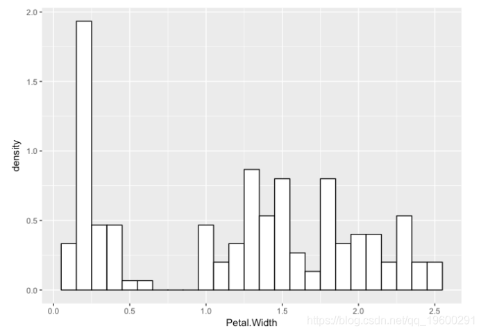
现在,让我们考虑一个花瓣宽度为鸢尾花的真实例子。
p <- ggplot(iris, aes(x = Petal.Width)) +
  geom_histogram(aes(x = Petal.Width, ..density..), binwidth = 0.1, colour = "black", fill = "white")
p

flexfit <- flexmix(Petal.Width ~ 1, data = iris, k = 3, model = list(mo1, mo2, mo3))

print(table(clusters(flexfit), iris$Species))
##
##     setosa versicolor virginica
##   1      0          2        46
##   2      0         48         4
##   3     50          0         0

geom_histogram(aes(x = Petal.Width, ..density..), binwidth = 0.1, colour = "black", fill = "white") +
                 args = list(c1[1], c1[2], lam[1]/sum(lam)),
                colour = "red", lwd = 1.5) +
stat_function(geom = "line", fun = plot_mix_comps,
                args = list(c2[1], c2[2], lam[2]/sum(lam)),
 stat_function(geom = "line", fun = plot_mix_comps,
                args = list(c3[1], c3[2], lam[3]/sum(lam)),
                colour = "green", lwd = 1.5) +
ylab("Density")
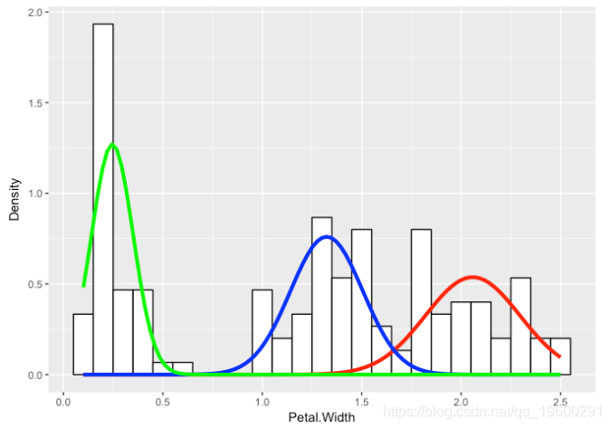

即使我们不知道潜在的物种分配,我们也能够对花瓣宽度的基本分布做出某些陈述 。
非常感谢您阅读本文,有任何问题请在下面留言!
1
1
关于作者
Kaizong Ye是拓端研究室(TRL)的研究员。
本文借鉴了作者最近为《R语言数据分析挖掘必知必会 》课堂做的准备。
 【视频】因子分析简介及R语言应用实例:对地区经济研究分析重庆市经济指标
 R语言宏观经济学:IS-LM曲线可视化货币市场均衡
 R语言代做编程辅导和解答GLM Coursework
 R语言分析上海空气质量数据:kmean聚类、层次聚类、时间序列分析:arima模型、指数平滑法